Abstract
What did i do?
I've measured my heart rate by using Fitbit Charge 5 and 4 simultaneously
How did i do it?
I've used bland altman plot approach to build agreement between 2 devices.
What did i learn?
Fitbit Charge 5 seems to be a biased for +0.6bpm versus Fitbit Charge 4. Devices doesnt agree well, with limits of agreement between -6.6 and 7.8 beats per minute. Trends are pretty consistent which is a good sign.
Introduction
Heart rate is important biomarker which represents general health. Accurate measurements may provide some useful insights in sickness and disease detection.
The purpose of this experiment (n=1) is to compare heart data between 2 wristworn devices.
Materials & Methods
Participants
Adult male anthropometrics was described in previous article.
Experimental design
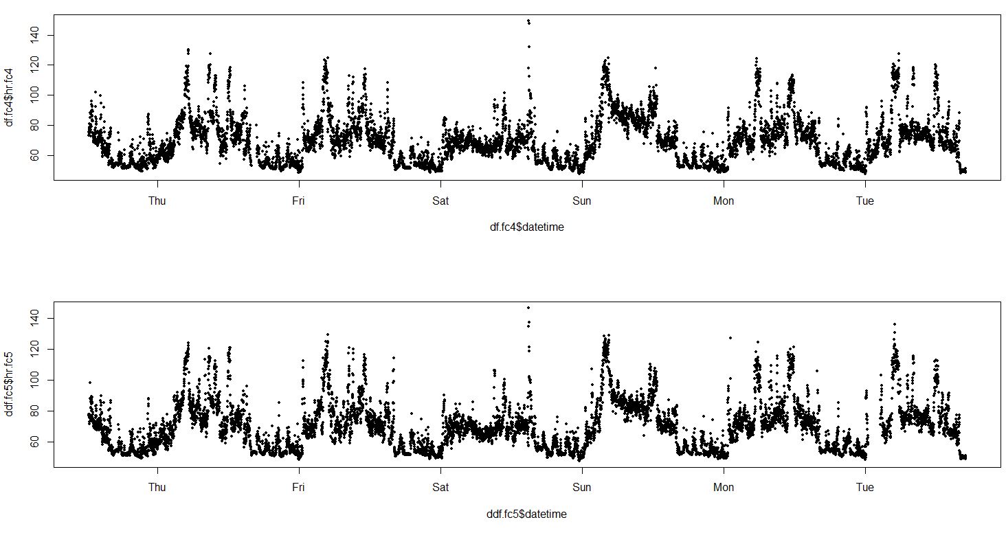
From 2021-10-06 to 2021-10-12 Fitbit Charge 5 and Charge 4 was weared on same hand (left) and heart rate data were collected. There were single training session (~20 minutes of rowing) and a few ~1 hour walks.
Results
To check heart rate agreement i've decided to build Bland-Altman plots. Heart rates were compared on same resolutions. There were total ~65000 measurements during that period.
Bland-Altman plot for 1 minute average heart rate:
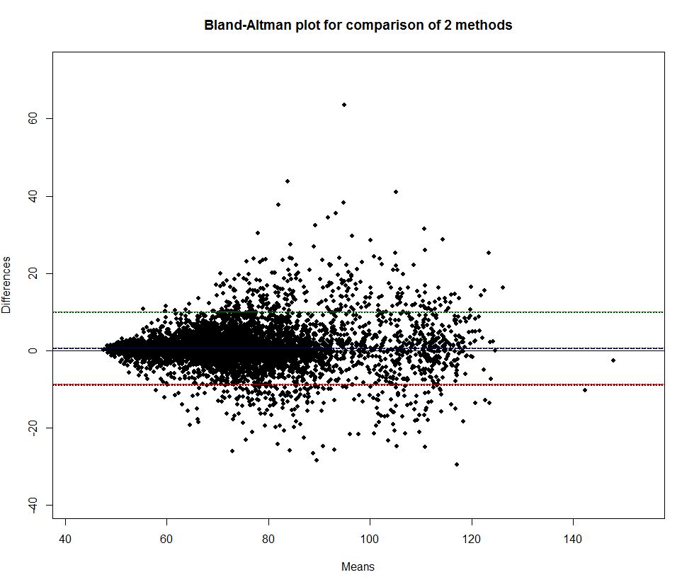
X and Y axis are in beats per minute
How to read this plot? Imagine we have a list of heart rate measuremens, n rows, each row contain 2 values one for FC4 and one for FC5. Then for each row we compute mean for both measures: (FC5 - FC4) / 2 and their difference (FC5 - FC4). Then we plot means on X and differences on Y.
For example, we can see that when heart rate is less than 60 bpm devices agree well (small difference FC5 - FC4). But when heart rate goes to 80 they agree less.
Black dashed line slightly above x axis indicate bias (difference between overall means). Green and red lines represents 95% limits of agreement.
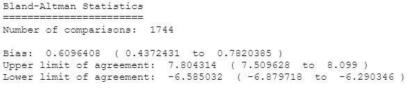
Here we can see 0.6 bpm bias and wide limits of agreement [-8.7,9.9]. Thats seems like a poor agreement.
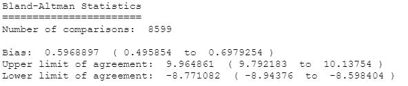
Lets build a linear regression:
Adjusted R-squared is a proportion of shared variance between both devices. We can see ~91% value which is not bad and is equal to correlation coefficient of 0.95. Devices seems to follow patterns pretty well, which is easily detected by visual inspection:
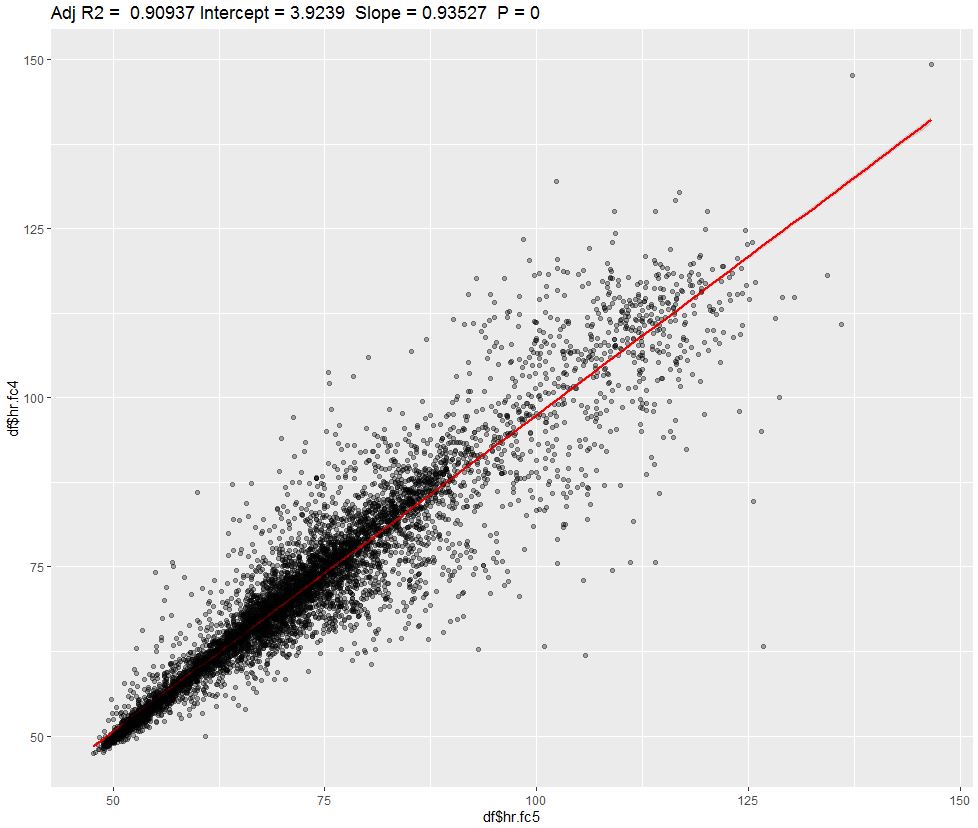
We can check how devices agree on 5 minute periods:
Limits of agreement were improved, but not too much.
Discussion
This data analysis suggests a poor agreement for absolute heart rate measurement value on 1-min and 5-min resolution windows. On the other side devices share 91% of variation (R-squared) and correlation coefficient is 0.95 is pretty large which suggests that devices follow similar trend pretty well.
Data availability & Information
Welcome for questions, suggestions and critics in comments below.
Original unmodified (exported) raw data for Fitbit Charge 5 here and for Fitbit Charge 4 is here.
alpha <- 0.05
source("https://blog.kto.to/uploads/r/functions.R")

df.fc4.raw <- na.omit(read.json.dir("Data/fc4/"))
df.fc4.raw <- df.fc4.raw[df.fc4.raw$value.confidence > 0, ]
df.fc4 <- data.frame(datetime = as.POSIXct(df.fc4.raw$dateTime, tryFormats = c("%m/%d/%y %H:%M:%OS")), hr = df.fc4.raw$value.bpm)

df.fc5.raw <- na.omit(read.json.dir("Data/fc5/"))
df.fc5.raw <- df.fc5.raw[df.fc5.raw$value.confidence > 0, ]
df.fc5 <- data.frame(datetime = as.POSIXct(df.fc5.raw$dateTime, tryFormats = c("%m/%d/%y %H:%M:%OS")), hr = df.fc5.raw$value.bpm)


library(lubridate)
library(dplyr)

df.fc4 = df.fc4 %>%
  mutate(datetime = floor_date(datetime, unit = "1 minute")) %>%
  group_by(datetime) %>%
  summarise(hr.fc4 = mean(hr, na.rm = TRUE))

df.fc5 = df.fc5 %>%
  mutate(datetime = floor_date(datetime, unit = "1 minute")) %>%
  group_by(datetime) %>%
  summarise(hr.fc5 = mean(hr, na.rm = TRUE))

par(mfrow = c(2,1))
plot(df.fc4$datetime, df.fc4$hr.fc4, pch = 20, cex = .9)
plot(df.fc5$datetime, df.fc5$hr.fc5, pch = 20, cex = .9)

df <- left_join(df.fc4, df.fc5, by=c("datetime"))
df <- na.omit(df)

library(blandr)
library(shiny)
library(boot)

blandr.statistics(df$hr.fc5, df$hr.fc4, sig.level = 1 - alpha, LoA.mode = 1)

par(mfrow = c(1,1))
blandr.draw(df$hr.fc5, df$hr.fc4, plotter = "rplot")
#blandr.output.report(df$hr.fc5, df$hr.fc4)


df$diff <- df$hr.fc5 - df$hr.fc4
summary(df$diff); quantile(df$diff, 0.025); quantile(df$diff, 0.975)

boot.fn <- function(data, indices) { return(mean(data[indices]))}
boot_results <- boot(df$diff, R = 1000, statistic = boot.fn); boot_results
boot.ci(boot_results, conf=1-alpha, type="perc")

lm.fit <- lm(df$hr.fc4 ~ df$hr.fc5)
summary(lm.fit)
par(mfrow = c(2,2))
plot(lm.fit)

library(car)
par(mfrow = c(1,1))
avPlots(lm.fit, ellipse = TRUE)

ggplotRegression(lm.fit)
Statistical analysis
RStudio version 1.3.959 and R version 4.0.2.