Accuracy - Oura ring 2.0 vs Dreem 2 EEG sleep staging

Abstract

What did i do?

I've measured my sleep data by using Oura ring and Dreem 2 EEG.

How did i do it?

I've used confusion matrix to reveal agreement between 2 devices.

What did i learn?

Oura ring sleep staging have a weak agreement ~60% with EEG device. I'll ignore oura sleep staging since it's accuracy is not enough for my experiments. Here is final agreement (diagonal line) if you dont have time to read:

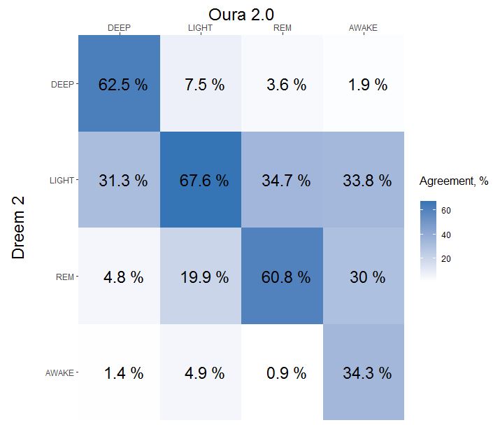
Updated at 22-01-2022 (sleep data: 1047 hours => 1987 hours)

Introduction

Sleep stages data may reveal some sleep disorders and may be used for sleep quality and quantity asessment. Oura ring algorithms determine sleep stages by using non-eeg data (hr, hrv, accelerometer) and their accuracy is questionable.

The purpose of this experiment (n=1) is to compared hypnogram data between finger worn device and eeg headband.

Materials & Methods

Participants

1 adult male (#1) anthropometrics was described in previous article and 1 adult female (#2).

Experimental design

From 2020-08-27 to 2021-09-16 sleep quality and quantity was assessed by Dreem 2 EEG Headband which was validated against gold standard PSG. At same time Oura ring was weared and sleep data was collected. There were 130 nights with data from both devices for male and 74 nights for female.

Results

To compare sleep accuracy i've decided to use confused matrix approach. Hypnograms were compared on same resolutions. There were total 1987 hours of data for #1 and i've decided not to build CI's because of large dataset.
Lets build a simplified confusion matrix plot:

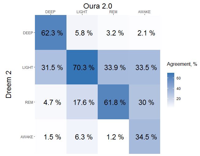
How to read confusion matrix? Columns belongs to Oura, rows belongs to Dreem, diagonal is agreement between both devices. In a 1st column we can see that 62.3% of oura DEEP sleep was recognized as DEEP sleep by Dreem 2, 31.5% of Oura DEEP was recognized as LIGHT by Dreem 2 and 4.7% of Oura DEEP was actually REM. Sum of each column is a 100%.

Oura detects correctly 62% of DEEP, misidentified part goes mostly to LIGHT (31%)
Oura detects correctly 70% of LIGHT, misidentified part goes mostly to REM (18%)
Oura detects correctly 62% of REM, misidentified part goes mostly to LIGHT(34%)
Oura detects correctly 34% of AWAKE, misidentified part mostly split between LIGHT(33%) and REM (30%)

Here is more detailed confusion matrix if anybody interested:

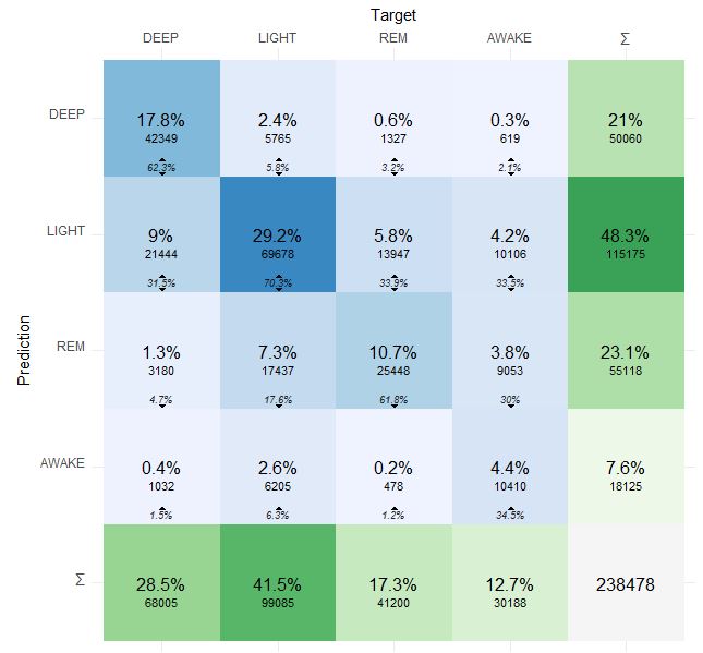
Prediction is Dreem 2 and Target is Oura 2.0.

	Oura	Dreem	Difference
DEEP	28.5%	21%	x1.35 overestimate
LIGHT	41.5%	48.3%	x1.15 underestimate
REM	17.3%	23.1%	x1.3 underestimate
AWAKE	12.7%	7.6%	x1.7 overestimate

Percentage base is Time in Bed = DEEP + LIGHT + REM. + AWAKE.

Anyway under/overestimations are of less interest because does not require stages predicted at correct time as at previous chart. These variations might be individual and not generalizable.

At 25 June Oura introduced new algorhitm for sleep staging and scientific validation of accuracy improved to 80%-90%. It's not released yet, but looks promising. Since sometimes there are gaps in night data even, i dont understand how can they reach accuracy claimed in paper in a real world conditions.

Results for #2

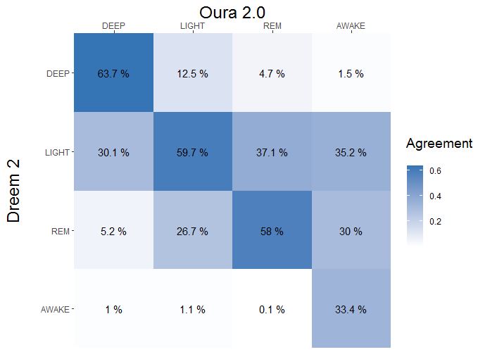
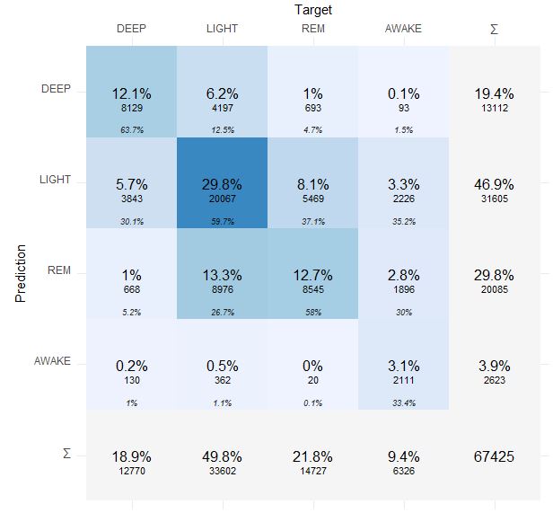
Pooled results #1 + #2

Cohen's Kappa is 0.43 representing a weak agreement:

Discussion

This data analysis suggests weak accuracy of sleep staging from Oura ring. Even awake time was detected with poor accuracy, meaning TST (which is of large interest) metric is also incorrect. It seems ring is good only in detection of TIB (Time in bed).

I'll ignore and will not use oura sleep staging data and TST in my experiments / data analysis since i need a good sensitivity for variations in sleep. In a present time i cant find a non-eeg devices with acceptable sleep staging.

Data availability & Information

Welcome for questions, suggestions and critics in comments below.

Original unmodified (exported) raw data for oura ring is here and for dreem is here.

library(stringr)
library(lubridate)
library(jsonlite)
library(dplyr)
library(plyr)
library(cvms)
library(e1071)

library(vcd)
library(caret)
library(modeest)
library(ggplot2)
library(iterators)
library(parallel)
library(doParallel)
registerDoParallel(cores=24)

#me
dreem <- read.csv("https://blog.kto.to/uploads/dreem-20-01-2022", skip = 5, sep = ';', header = TRUE)
rawoura<-fromJSON('https://blog.kto.to/uploads/oura_2022-01-22T01-03-35.json')

#wife
#dreem <- read.csv("https://blog.kto.to/uploads/p2-dreem.csv", skip = 5, sep = ';', header = TRUE)
#rawoura<-fromJSON('https://blog.kto.to/uploads/p2-oura_2021-09-22T11-26-20.json')

#process dreem hypnogram
dreem <- dreem[!is.na(dreem$Type),]
dreem$Hypnogram <- str_replace(dreem$Hypnogram, "\\[", "")
dreem$Hypnogram <- str_replace(dreem$Hypnogram, "\\]", "")
dreem$Hypnogram <- str_replace_all(dreem$Hypnogram, "WAKE", "4")
dreem$Hypnogram <- str_replace_all(dreem$Hypnogram, "REM", "3")
dreem$Hypnogram <- str_replace_all(dreem$Hypnogram, "Light", "2")
dreem$Hypnogram <- str_replace_all(dreem$Hypnogram, "Deep", "1")
dreem$HypnogramList <- str_split(dreem$Hypnogram, ",")
dreem$datetime <- ymd_hms(dreem$Start.Time)

dreem <- dreem[dreem$Start.Time != "2021-08-18T23:01:04+07:00",] #battery went out in the middle of night

dreem <- dreem[dreem$Start.Time != "2021-10-01T00:15:49+07:00",] #battery went out in the middle of night

dreem <- dreem[dreem$Start.Time != "2021-10-14T23:15:49+07:00",] #battery went out in the middle of night

dreem <- dreem[dreem$Start.Time != "2022-01-13T23:27:38+07:00",] #battery went out in the middle of night


dreems <- dreem

results <- foreach(i=1:nrow(dreems), .combine='rbind', .multicombine=TRUE, .packages = "lubridate") %dopar% {
  ddf = NULL
  for (j in 1:length(dreems$HypnogramList[i][[1]]))
  {
    stage <- as.numeric(dreems$HypnogramList[i][[1]][j])
    datetime <- dreems$datetime[i] + 30 * (j - 1)
    res <- c(datetime = datetime, stage = stage)
    ddf = rbind(ddf, res)
  }
  return(ddf)
}
  
dreem_data <- as.data.frame(results)
row.names(dreem_data) <- NULL
summary(dreem_data)

#process oura hypnogram
oura <- flatten(data.frame(rawoura$sleep))
oura$datetime <- ymd_hms(oura$bedtime_start)
ouras <- oura

oura_results <- foreach(i=1:nrow(ouras), .combine='rbind', .multicombine=TRUE, .packages = "lubridate") %dopar% {
  odf = NULL
  for(j in 1:nchar(ouras$hypnogram_5min[i])) 
  {
    stage <- as.numeric(substring(ouras$hypnogram_5min[i], j, j)[1])
    for(k in 1:10) #downsample to 30-sec like dreem
    {
      datetime <- ouras$datetime[i] + 300 * (j - 1) + (k - 1)*30
      res <- c(datetime = datetime, stage = stage)
      odf = rbind(odf, res) 
    }
  }
  return(odf)
}

oura_data <- as.data.frame(oura_results)
row.names(oura_data) <- NULL
summary(oura_data)

#round datas for both hypnograms
period <-  "30s"
oura_data$dt <- as.POSIXct(oura_data$datetime, origin="1970-01-01")
oura_data$period <- round_date(oura_data$dt, period)
dreem_data$dt <- as.POSIXct(dreem_data$datetime, origin="1970-01-01")
dreem_data$period <- round_date(dreem_data$dt, period)

#merge data
merged_hypnogram <- inner_join(as.data.frame(oura_data[,c("period","stage")]), as.data.frame(dreem_data[,c("period","stage")]) , by = c("period" = "period"))
colnames(merged_hypnogram) <- c("datetime","oura","dreem")

merged_hypnogram <- merged_hypnogram[!is.na(merged_hypnogram$oura),]
merged_hypnogram <- merged_hypnogram[!is.na(merged_hypnogram$dreem),]

merged_hypnogram$dreem[merged_hypnogram$dreem == 1] <- "DEEP";
merged_hypnogram$dreem[merged_hypnogram$dreem == 2] <- "LIGHT";
merged_hypnogram$dreem[merged_hypnogram$dreem == 3] <- "REM";
merged_hypnogram$dreem[merged_hypnogram$dreem == 4] <- "AWAKE";

merged_hypnogram$oura[merged_hypnogram$oura == 1] <- "DEEP";
merged_hypnogram$oura[merged_hypnogram$oura == 2] <- "LIGHT";
merged_hypnogram$oura[merged_hypnogram$oura == 3] <- "REM";
merged_hypnogram$oura[merged_hypnogram$oura == 4] <- "AWAKE";

category_order <- c("DEEP", "LIGHT", "REM", "AWAKE") 
merged_hypnogram$oura = factor(merged_hypnogram$oura, levels = category_order)
merged_hypnogram$dreem = factor(merged_hypnogram$dreem, levels = category_order)

cm <- confusion_matrix(targets = as.factor(merged_hypnogram$oura), predictions = as.factor(merged_hypnogram$dreem))

#cmm1 <- cm
#cmm2 <- cm
#tb <- as.matrix(cmm1$Table[[1]], rownames = F) + as.matrix(cmm2$Table[[1]], rownames = F)
#Kappa(tb)

plot_confusion_matrix(cm$`Confusion Matrix`[[1]], 
                      place_x_axis_above = T,
                      add_row_percentages = F,
                      add_col_percentages = T,
                      rotate_y_text = F,
                      class_order = c("AWAKE", "REM", "LIGHT", "DEEP"),
                      add_sums = T)

cm <- table(merged_hypnogram$oura,merged_hypnogram$dreem)
#cm1 <- cm
#cm2 <- cm
#cm <- cm1 + cm2
cm <- cm / rowSums(cm)
cm <- as.data.frame(cm, stringsAsFactors = TRUE)
cm$Var2 <- factor(cm$Var2, rev(levels(cm$Var2)))

ggplot(cm, aes(Var1, Var2, fill = round(100*Freq,1))) +
  geom_tile() +
  geom_text(aes(label = paste(" ", round(100*Freq,1),"%")),  size=6) +
  scale_x_discrete(expand = c(0, 0),position = 'top') +
  scale_y_discrete(expand = c(0, 0),position = 'left') + 
  scale_fill_gradient(low = "white", high = "#3575b5") +
  labs(x = "Oura 2.0", y = "Dreem 2", fill = "Agreement, %") + 
  theme(legend.title = element_text(size = 12, margin = margin(0, 20, 10, 0)),
        axis.title.x = element_text(margin = margin(20, 20, 20, 20), size = 18),
        axis.title.y = element_text(margin = margin(0, 20, 0, 10), size = 18))

Statistical analysis

RStudio version 1.3.959 and R version 4.0.2. Cohen's Kappa interpretation reference