Abstract

What did i do?

I've measured my training load, steps and positive/negative emotions to find out if physical activity increases my mood.

How did i do it?

I've assessed my emotions using PANAS questionnaire, step count using Oura ring and training load using session RPE approach on a daily basis.

What did i learn?

Physical activity significantly increases my positive emotions and decrease negative emotions. 1 hour of moderate intensity training / 10 000 steps is enough to get a valuable effect.

Introduction

There is a some scientific evidence that exercise and intraday activity may increase mood.

The purpose of this observational data analysis (n=1) is to find if sRPE training load and steps can increase positive affect and decrease negative affect.

Materials & Methods

Participants

Adult male (n=1) anthropometrics was described in previous article

Experimental design

From 2020-09-19 to 2021-08-26 (294 days) daily training load (session RPE) and positive affect domain of PANAS was assessed.

Positive Affect of PANAS consists of 10 items with 5-point LikeRT, same for Negative Affect

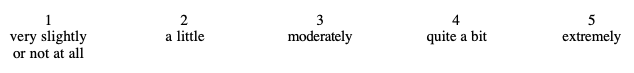
Sum of 10 items defines the Positive Affect score, ranging from 10 to 50 which was used in analysis.

Physical activity was calculated by using sRPE approach, described here. In a short, a time duration and Rating of Perceived Exertion on a 10-item scale was assessed for each physical activity (walking, running, cycling etc) withing 10 minutes after cessation. Multiplication of RPE and duration is a sRPE score in arbitrary units. Sum of all activities sRPE scores for given day was used in analysis. Daily step count were measured by Oura ring and multiplied by 0.85. It is important to note that sRPE approach includes daily steps.

Subjective sleep quality, mood, depression, anxiety, stress, fatigue and sleepiness was assessed by a popular in scientific research questionnaires described in previous experiment

Results

The data summary shown below

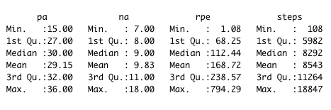
rpe (sRPE) in arbitrary units

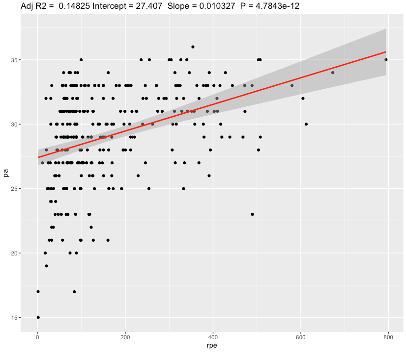
Linear regression, Positive Affect

	effect	p-adjusted	effect size
sRPE, m	0.01032	<0.0001*	moderate
Steps	0.000345	<0.0001*	weak

We can see a slope of 0.01 increase in Positive Affect scale for each additional 1 au of sRPE. Confidence for slope is very narrow [0.0104,0.0106] and effect size is Moderate.

Most of the days physical activity (sRPE) is about 110 au (median). 1 hour training with RPE score of 6 will add a 60 * 6 = 360 au of sRPE, which results in increasing Positive Affect by 360 * 0.01 = 3.6 points.

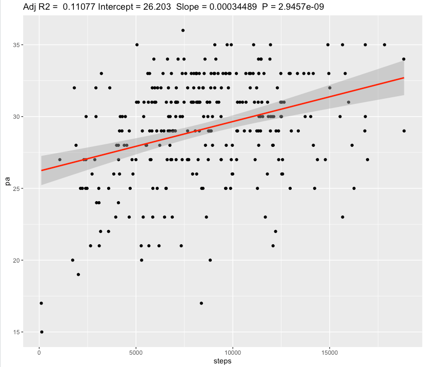
Also we can see a slope of 0.00034 increase in Positive Affect scale for each additional 1 step or a 0.34 for each 1000 steps. Confidence for slope is very narrow [0.000341  0.000348] and effect size is Weak.

Even with weak effect size, additional 3.4 Positive Affect points for 10 000 steps day seems to be valuable.

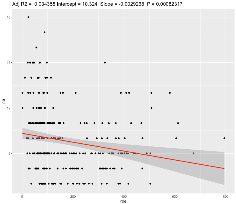
Linear regression, Negative Affect

	effect	p-adjusted	effect size
sRPE, m	-0.0029	<0.0008*	weak
Steps	-0.000152	<0.0001*	weak

We can see a slope of 0.003 decrease in Negative Affect scale for each additional 1 au of sRPE. Confidence for slope is very narrow [-0.00298,-0.00287] and effect size is Weak.

Even with weak effect size, 1 hour training with RPE score of 6 will add a 60 * 6 = 360 au of sRPE, which results in decreasing Negative Affect by 360 * 0.003 = 1.1 points, which seems to be valueable.

Also we can see a slope of -0.000152 decrease in Negative Affect scale for each additional 1 step or a -0.15 for each 1000 steps. Confidence Interval for slope is very narrow
[-0.000154,-0.000150] and effect size is Weak.

Even with weak effect size, decrease by -1.5 in Negative Affect points for 10 000 steps day seems to be valuable.

Discussion

The main result of this experiment is a statistically significant association between physical activity and positive/negative emotions with a moderate/weak effect sizes.
Increasing Positive Affect by 3-4 points by adding medium intensive training or getting 10 000 steps per day is seems to be a beneficial for general mood and happyness. My most positive days is PA from 33 to 36, average day is 29 - 30 and just 1 good training or a lot of walking during average day pushing my mood into most positive days. Same applies for Negative affect.

In conclusion, these results points me to keep my training load at high levels but at the same keeping eye in overtraining. In this paradigm, knowing how not to overtrain becomes very important. During non-training taking a 10k steps per day seems to be important.

Limitations:

• These results are NOT generalizable
• Absence of blinding, randomization, observational nature, n=1
• Often correlation ≠ causation
• Questionnaires widely used in research are prone to participant bias.
• There is a lot of other factors affecting mood (sleep, diet, caffeine etc) which not taken into account

Data availability & Information

Welcome for questions, suggestions and critics in comments below.

Data is fully available here

library(effectsize)
library(lubridate)
library(ggplot2)


ggplotRegression <- function (fit) {
 
  require(ggplot2)
 
  ggplot(fit$model, aes_string(x = names(fit$model)[2], y = names(fit$model)[1])) +
    geom_point() +
    stat_smooth(method = "lm", col = "red") +
    labs(title = paste("Adj R2 = ",signif(summary(fit)$adj.r.squared, 5),
                       "Intercept =",signif(fit$coef[[1]],5 ),
                       " Slope =",signif(fit$coef[[2]], 5),
                       " P =",signif(summary(fit)$coef[2,4], 5)))
}


tlpa <- read.csv("https://blog.kto.to/uploads/pa-na-rpe-sick-food-step-sauna-meditation.csv")
tlpa <- tlpa[!is.na(tlpa$`pa`),]
tlpa <- tlpa[!is.na(tlpa$`steps`),]
tlpa <- tlpa[!is.na(tlpa$`rpe`),]
summary(tlpa)

l <- lm(cbind(pa, na) ~ rpe, data=tlpa)
summary(anova(l))
s <- summary(l); s
interpret_r2(s$`Response pa`$adj.r.squared[1])
interpret_r2(s$`Response na`$adj.r.squared[1])
confint(l , level = 0.05)

l2 <- lm(cbind(pa, na) ~ steps, data=tlpa)
summary(anova(l2))
s2 <- summary(l2); s2
interpret_r2(s2$`Response pa`$adj.r.squared[1])
interpret_r2(s2$`Response na`$adj.r.squared[1])
confint(l2 , level = 0.05)


ggplotRegression(lm(pa ~ rpe, data=tlpa))
ggplotRegression(lm(na ~ rpe, data=tlpa))
ggplotRegression(lm(pa ~ steps, data=tlpa))
ggplotRegression(lm(na ~ steps, data=tlpa))

p.adjust(c(
  s$`Response pa`$coefficients[,4][2],
  s2$`Response pa`$coefficients[,4][2]), method="BH")


p.adjust(c(
  s$`Response na`$coefficients[,4][2],
  s2$`Response na`$coefficients[,4][2]), method="BH")Response pa :

Call:
lm(formula = pa ~ rpe, data = tlpa)

Residuals:
     Min       1Q   Median       3Q      Max
-12.4210  -1.8578   0.5336   2.5439   6.5682

Coefficients:
             Estimate Std. Error t value Pr(>|t|)    
(Intercept) 27.407285   0.314102  87.256  < 2e-16 ***
rpe          0.010327   0.001432   7.211 4.78e-12 ***
---
Signif. codes:  0 ‘***’ 0.001 ‘**’ 0.01 ‘*’ 0.05 ‘.’ 0.1 ‘ ’ 1

Residual standard error: 3.441 on 292 degrees of freedom
Multiple R-squared:  0.1512,    Adjusted R-squared:  0.1483
F-statistic:    52 on 1 and 292 DF,  p-value: 4.784e-12


Response na :

Call:
lm(formula = na ~ rpe, data = tlpa)

Residuals:
    Min      1Q  Median      3Q     Max
-3.2189 -1.2638 -0.2921  0.9587  7.7486

Coefficients:
              Estimate Std. Error t value Pr(>|t|)    
(Intercept) 10.3237482  0.1899149   54.36  < 2e-16 ***
rpe         -0.0029268  0.0008659   -3.38 0.000823 ***
---
Signif. codes:  0 ‘***’ 0.001 ‘**’ 0.01 ‘*’ 0.05 ‘.’ 0.1 ‘ ’ 1

Residual standard error: 2.081 on 292 degrees of freedom
Multiple R-squared:  0.03765,    Adjusted R-squared:  0.03436
F-statistic: 11.43 on 1 and 292 DF,  p-value: 0.0008232


> interpret_r2(s$`Response pa`$adj.r.squared[1])
[1] "moderate"
(Rules: cohen1988)
> interpret_r2(s$`Response na`$adj.r.squared[1])
[1] "weak"
(Rules: cohen1988)
> confint(l , level = 0.05)
                     47.5 %       52.5 %
pa:(Intercept) 27.387571327 27.426997900
pa:rpe          0.010236981  0.010416739
na:(Intercept) 10.311828971 10.335667352
na:rpe         -0.002981136 -0.002872449