Abstract
What did i do?
I've measured my core body temperature circadian rhythm, to make sure it's present and is not disturbed (i've had a few years of shift work 10 years ago).
How did i do it?
I've used iButton placed in armpit and MetaMotionR placed at open part of wrist to measure exposure to ambient light, for 2 weeks.
What did i learn?
My body temperature circadian rhythm is present and looks strong enough.
Introduction
Circadian rhythm disorders may decrease our healthspan and increase occurrence of chronic diseases during aging.
The purpose of this experiment (n=1) is to find diurnal changes in body temperature.
Materials & Methods
Participants
Adult male (n=1) anthropometrics was described in previous article
Experimental design
From 2020-08-20 to 2020-09-04 (14 days) body temperature was measured by iButton placed inside armpit, covered by medical adhesive patch. iButton was taken out for shower / swimming activities and after finishing patch was re-applied.
Ambient light in lux was measured by MetaMotionR placed at the open part of a wrist.
Results
Visual inspection of data reveals circadian rhythm:
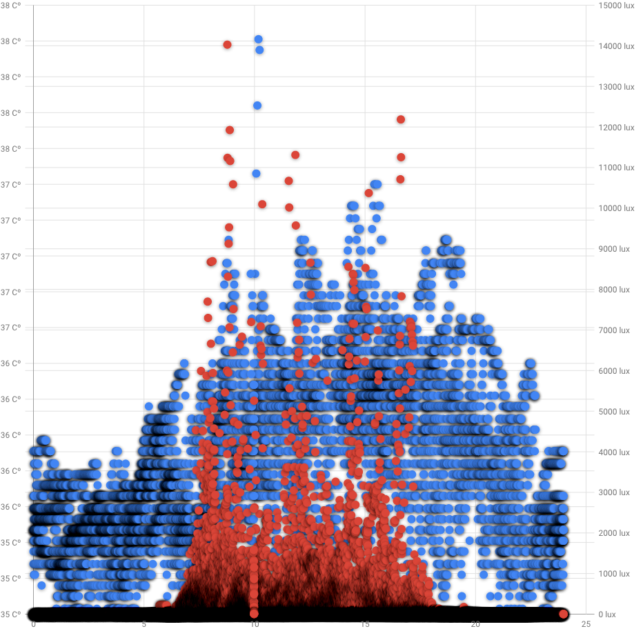
Blue dots is a armpit temperature in celsius (left Y axis), red is ambient light in lux (right Y axis). X axis is a hour of a day. Google Developer charts for some reasons doesnt show decimal point for temperature and adding empty 25 hour. Measurements density highlighted by shadowing.
Day vs Night temperature
| Mean | 95% CI for Mean | |
| Night (21:00 - 7:00) | 35.56℃ | [35.55,35.57] |
| Day (9:00 - 19:00) | 36.13℃ | [36.12,36.14] |
Confidence intervals a pretty narrow and far away enough to prove statistically significant difference between day and night.
Group differences
| Effect size | 95% CI | |
| Hedges g | Large | [-1.673,-1.673] |
| Mean difference | -0.5716℃ | [-0.5716, -0.5716] |
We can see a pretty narrow (n~5000) CI's showing a difference of 0.57℃ between day and night with "Large" effect size.
Discussion
The main result of that experiment is 0.57℃ difference between day and night which acts as a proxy of my circadian rhythm strength. I'll continue checking it in future, to see the trends.
Data availability & Information
Welcome for questions, suggestions and critics in comments below.
Data is fully available here.
R Code:
library(goftest)
library(dplyr)
library(effectsize)
library(lubridate)
library(ggplot2)
library(boot)
library(bootES)

temp <- read.csv("https://blog.kto.to/uploads/circadian-ibutton.csv")
temp <- temp[!is.na(temp$armpittemp),]

#filter 21:00 - 7:00 as group 1, 9:00 - 19:00 as group 2, other as group 0
temp <- temp %>% select(datetime,armpittemp)  %>%
  mutate(group = if_else(((hour(datetime) >= 21) | (hour(datetime) <=  7)), 1,
                 if_else(((hour(datetime) <= 19) & (hour(datetime) >=  9)),2, 0)));

#remove group 0
temp <- temp[temp$group != 0,]

#check for normality distribution
st <-ad.test(temp$armpittemp) #shapiro.test for n < 5000,  ad.test othervise
if_else(st$p.value < 0.05, 'non-uniform distribution', 'uniform distribution')

bootMean <- function(data, i) { d <- data[i]; return(mean(d)); }
bootMeanDiff <- function(data, i)
{
  d <- data;
  data_group1 <- !is.na(d$group)&d$group == 1
  data_group2 <- !is.na(d$group)&d$group == 2
  g1 <- d$armpittemp[data_group1]
  g2 <- d$armpittemp[data_group2]
  return(mean(g1) - mean(g2));
}
bootHedgesG <- function(data, i) #calc hedges G to measure effect sizes
{
  d <- data;
  data_group1 <- !is.na(d$group)&d$group == 1
  data_group2 <- !is.na(d$group)&d$group == 2
  g1 <- d$armpittemp[data_group1]
  g2 <- d$armpittemp[data_group2]
  h <- hedges_g(g1, g2)
  return(h$Hedges_g[1]);
}

#bootstrap hedges G effect size between group 1 and 2
results <- boot(data=temp, statistic=bootHedgesG, R=10000)
boot_result <- boot.ci(results, type = c("perc")); boot_result;
interpret_g(1.673, "cohen1988");

#bootstrap mean difference between group 1 and 2
results <- boot(data=temp, statistic=bootMeanDiff, R=10000)
boot_result <- boot.ci(results, type = c("perc")); boot_result;
interpret_g(1.673, "cohen1988");


#take out group 1 and 2 from dataset
data_group <- !is.na(temp$group)&temp$group == 1
day <- temp$armpittemp[data_group]

data_group <- !is.na(temp$group)&temp$group == 2
night <- temp$armpittemp[data_group]

#calc averages & CI
results <- boot(data=day, statistic=bootMean, R=10000)
day_result <- boot.ci(results, type = c("perc")); day_result;

results <- boot(data=night, statistic=bootMean, R=10000)
night_result <- boot.ci(results, type = c("perc")); night_result;
[1] "non-uniform distribution"BOOTSTRAP CONFIDENCE INTERVAL CALCULATIONS
Based on 10000 bootstrap replicates
CALL :
boot.ci(boot.out = results, type = c("perc"))
Intervals :
Level Percentile
95% (-1.673, -1.673 )
Calculations and Intervals on Original ScaleBased on 10000 bootstrap replicates
CALL :
boot.ci(boot.out = results, type = c("perc"))
Intervals :
Level Percentile
95% (35.55, 35.57 )
Calculations and Intervals on Original Scale
Based on 10000 bootstrap replicates
CALL :
boot.ci(boot.out = results, type = c("perc"))
Intervals :
Level Percentile
95% (36.12, 36.14 )
Calculations and Intervals on Original Scale
BOOTSTRAP CONFIDENCE INTERVAL CALCULATIONS
Based on 10000 bootstrap replicates

CALL :
boot.ci(boot.out = results, type = c("perc"))

Intervals :
Level     Percentile
95%   (-0.5716, -0.5716 )
Calculations and Intervals on Original Scale
Statistical analysis
RStudio version 1.3.959 and R version 4.0.2. Confidence Intervals was build using bootstrap. Effect sizes based on Hedge's g, Cohen's 1988 rules