Abstract

What did i do?

I've measured my HRV to find out if it is a useful indicator of sickness and have value in early sickness detection and indication of recovery.

How did i do it?

I've assessed morning sickness score, nightly HRV by using Oura ring and morning standing HRV by using Polar H10. Daily and 7-day rolling averages was used.

What did i learn?

Sickness substantially decreases my standing HRV and showing moderate decrease in my nightly HRV. Daily morning standing HRV seems to be more sensitive than nightly values and provides valuable feedback of sickness status. Standing RMSSD seems to be a useful tool which provides insights about illness onset and recovery and helps make a decision of resuming physical activity. Nightly RMSSD values also provides insights on sickness status, but less sensitive.

Introduction

There is a some evidence that sickness cause drop in HRV.

The purpose of this observational data analysis (n=1) is to find if sickness causing decrease HRV.

Materials & Methods

Participants

Adult male (n=1) anthropometrics was described in previous article

Experimental design

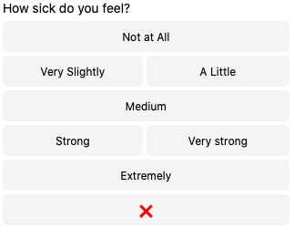
From 2020-09-19 to 2021-09-01 (284 days) subjective sickness score was assessed by using 1-item 7-point Likert scale (0-6) every morning and evening:

Nightly HRV (RMSSD) was measured by Oura ring on a daily basis. 7-day rolling averages was calculated. Daily and 7-day values were log-transformed.

Morning HRV (RMSSD) was measured by Polar H10 in Kubios HRV app, after emptying urinary bladder, within 5 minutes after waking up. Stabilization period was 1 minute and measurement duration was 1 minute. 7-day rolling averages was calculated. Daily and 7-day values were log-transformed.

Results

Sickness and HRV

Visual inspection of sickness status, daily RMSSD and 7D rolling averages.

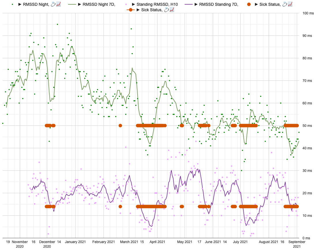
Sickness status (red circles) for days with sickness score >= 6. Lines representing 7d rolling averages and points for daily values. Green for nightly and violet for standing values.

As we can see, HRV seems to drop significantly during sickness.

The data summary shown below

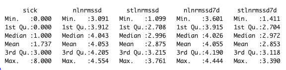
sick is a sum of morning and evening scores. nlnmrssd - nightly ln(RMSSD). nlnmrssd7d - 7-day rolling average of nightly ln(RMSSD), stlnmrssd - morning standing ln(RMSSD). stlnmrssd7d - 7-day rolling average of morning standing ln(RMSSD).

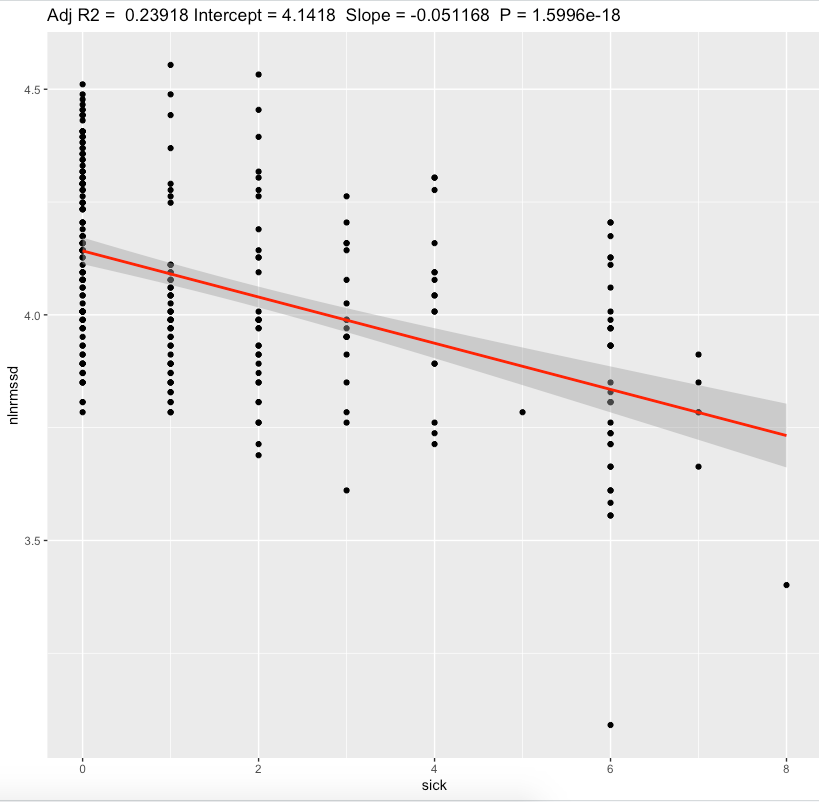
Linear regression, Sick score

	effect	p-adjusted	effect size
nightly ln(RMSSD)	-0.051	<0.0001*	moderate
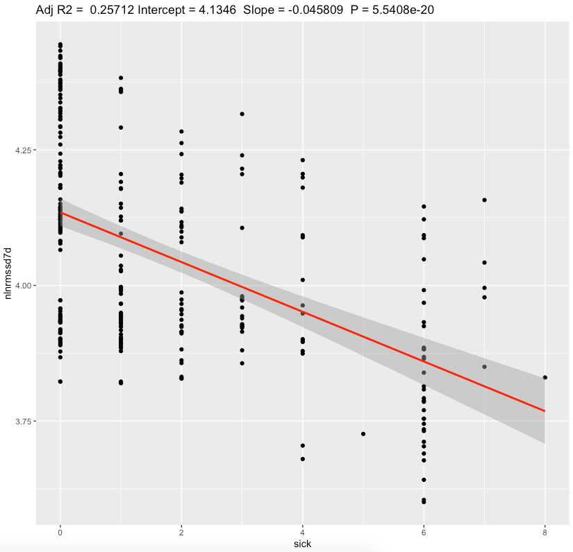
nightly 7d ln(RMSSD)	-0.046	<0.0001*	moderate
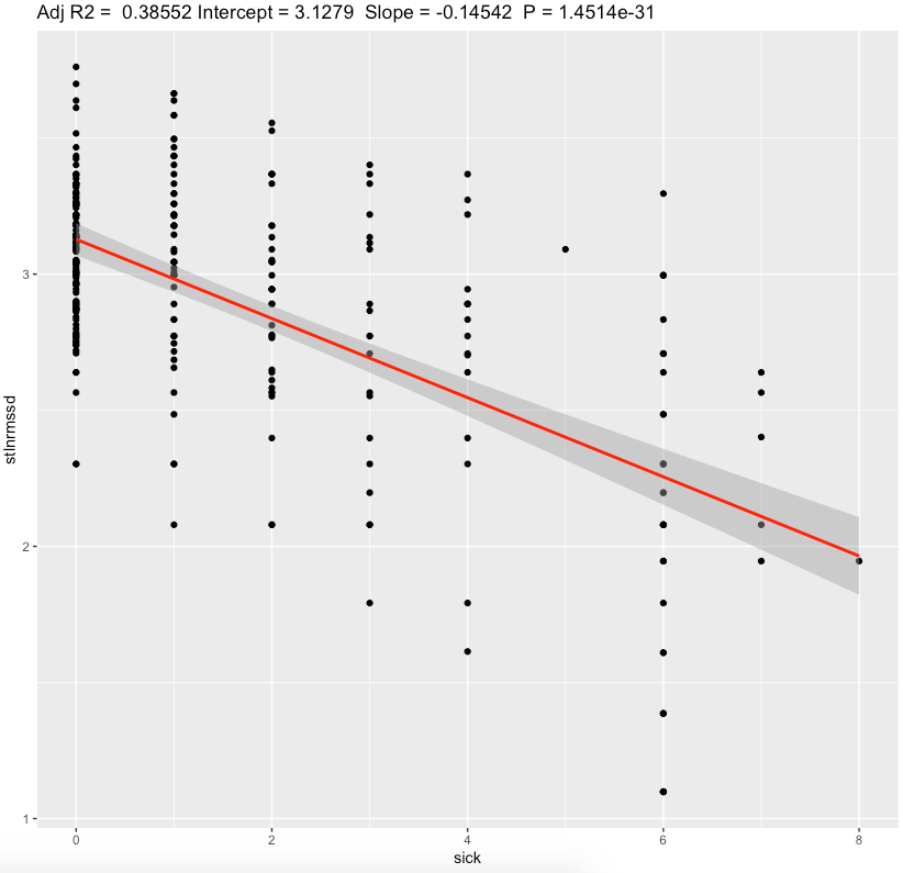
standing ln(RMSSD)	-0.145	<0.0001*	substantial
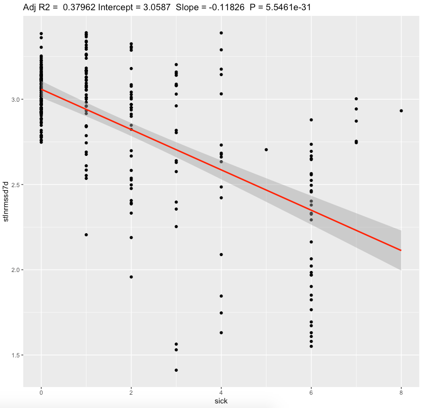
standing 7d ln(RMSSD)	-0.118	<0.0001*	substantial

We can see a moderate effect slopes for nightly values and substantial effect on a standing values. Morning standing RMSSD seems to be most sensitive to sickness status. Since my average standing ln(RMSSD) is 2.88 which is equivalent of RMSSD 17.8 ms, each 1 sickness point desceasing it by ~2.5 ms.

Discussion

The main result of this experiment is a statistically significant association between HRV and sickness with moderate/substantial effect sizes.

For 4-6 sickness score representing illness, standing RMSSD drop by ~10-15ms seems to be a huge. Nightly values are less sensitive.

In conclusion, these results points me to continue to measure my morning standing HRV and use it as possible indication of sickness onset and recovery status after illness. In my case, i prefer a standing HRV because of bigger sensitivy to sickness compared with nightly values.

Limitations:

• These results are NOT generalizable
• Absence of blinding, randomization, observational nature, n=1
• Often correlation ≠ causation
• Questionnaires widely used in research are prone to participant bias.
• There is a lot of other factors affecting HRV (sleep, diet, caffeine etc) which not taken into account

Data availability & Information

Welcome for questions, suggestions and critics in comments below.

Data is fully available here

library(dplyr)
library(lubridate)
library(effectsize)
library(jsonlite)


ggplotRegression <- function (fit) {
 
  require(ggplot2)
 
  ggplot(fit$model, aes_string(x = names(fit$model)[2], y = names(fit$model)[1])) +
    geom_point() +
    stat_smooth(method = "lm", col = "red") +
    labs(title = paste("Adj R2 = ",signif(summary(fit)$adj.r.squared, 5),
                       "Intercept =",signif(fit$coef[[1]],5 ),
                       " Slope =",signif(fit$coef[[2]], 5),
                       " P =",signif(summary(fit)$coef[2,4], 5)))
}



daily <- read.csv("https://blog.kto.to/uploads/pa-na-rpe-sick-food-step-sauna-meditation-hrv.csv")
daily <- daily[!is.na(daily$`sick`),]
daily <- daily[!is.na(daily$`rpe`),]
daily <- daily[!is.na(daily$`rpe7d`),]
daily <- daily[!is.na(daily$`nlnrmssd`),]
daily <- daily[!is.na(daily$`nlnrmssd7d`),]
daily <- daily[!is.na(daily$`stlnrmssd`),]
daily <- daily[!is.na(daily$`stlnrmssd7d`),]

daily$pa = NULL
daily$na = NULL
daily$food = NULL
daily$steps = NULL
daily$sauna = NULL
daily$meditation = NULL
daily$rpe = NULL
daily$rpe7d = NULL
summary(daily)

l <- lm(cbind(nlnrmssd, nlnrmssd7d, stlnrmssd, stlnrmssd7d) ~ sick, data=daily)
summary(daily)
summary(anova(l))
s <- summary(l); s
interpret_r2(s$`Response nlnrmssd`$adj.r.squared[1])
interpret_r2(s$`Response nlnrmssd7d`$adj.r.squared[1])
interpret_r2(s$`Response stlnrmssd`$adj.r.squared[1])
interpret_r2(s$`Response stlnrmssd7d`$adj.r.squared[1])

p.adjust(c(
  s$`Response nlnrmssd`$coefficients[,4][2],
  s$`Response nlnrmssd7d`$coefficients[,4][2],
  s$`Response stlnrmssd`$coefficients[,4][2],
  s$`Response stlnrmssd7d`$coefficients[,4][2]
  ), method="BH")

confint(l , level = 0.05)

ggplotRegression(lm(nlnrmssd ~ sick, data=daily))
ggplotRegression(lm(nlnrmssd7d ~ sick, data=daily))
ggplotRegression(lm(stlnrmssd ~ sick, data=daily))
ggplotRegression(lm(stlnrmssd7d ~ sick, data=daily))

c <- cor.test(daily$nlnrmssd, daily$sick); c
interpret_r(c$estimate[[1]][1], "cohen1988")

c <- cor.test(daily$nlnrmssd7d, daily$sick); c
interpret_r(c$estimate[[1]][1], "cohen1988")

c <- cor.test(daily$stlnrmssd, daily$sick); c
interpret_r(c$estimate[[1]][1], "cohen1988")

c <- cor.test(daily$stlnrmssd7d, daily$sick); c
interpret_r(c$estimate[[1]][1], "cohen1988")
Response nlnrmssd :

Call:
lm(formula = nlnrmssd ~ sick, data = daily)

Residuals:
     Min       1Q   Median       3Q
-0.74376 -0.13448 -0.01468  0.14865
     Max
 0.49312

Coefficients:
             Estimate Std. Error t value
(Intercept)  4.141813   0.014973 276.627
sick        -0.051168   0.005423  -9.435
            Pr(>|t|)    
(Intercept)   <2e-16 ***
sick          <2e-16 ***
---
Signif. codes:  
  0 ‘***’ 0.001 ‘**’ 0.01 ‘*’ 0.05 ‘.’
  0.1 ‘ ’ 1

Residual standard error: 0.1951 on 279 degrees of freedom
Multiple R-squared:  0.2419,    Adjusted R-squared:  0.2392
F-statistic: 89.03 on 1 and 279 DF,  p-value: < 2.2e-16


Response nlnrmssd7d :

Call:
lm(formula = nlnrmssd7d ~ sick, data = daily)

Residuals:
     Min       1Q   Median       3Q
-0.31194 -0.14468 -0.01718  0.13901
     Max
 0.34346

Coefficients:
            Estimate Std. Error t value
(Intercept)  4.13461    0.01278 323.474
sick        -0.04581    0.00463  -9.895
            Pr(>|t|)    
(Intercept)   <2e-16 ***
sick          <2e-16 ***
---
Signif. codes:  
  0 ‘***’ 0.001 ‘**’ 0.01 ‘*’ 0.05 ‘.’
  0.1 ‘ ’ 1

Residual standard error: 0.1666 on 279 degrees of freedom
Multiple R-squared:  0.2598,    Adjusted R-squared:  0.2571
F-statistic: 97.91 on 1 and 279 DF,  p-value: < 2.2e-16


Response stlnrmssd :

Call:
lm(formula = stlnrmssd ~ sick, data = daily)

Residuals:
     Min       1Q   Median       3Q
-1.15678 -0.22902  0.01324  0.23149
     Max
 1.04044

Coefficients:
            Estimate Std. Error t value
(Intercept)  3.12791    0.03021  103.55
sick        -0.14542    0.01094  -13.29
            Pr(>|t|)    
(Intercept)   <2e-16 ***
sick          <2e-16 ***
---
Signif. codes:  
  0 ‘***’ 0.001 ‘**’ 0.01 ‘*’ 0.05 ‘.’
  0.1 ‘ ’ 1

Residual standard error: 0.3936 on 279 degrees of freedom
Multiple R-squared:  0.3877,    Adjusted R-squared:  0.3855
F-statistic: 176.7 on 1 and 279 DF,  p-value: < 2.2e-16


Response stlnrmssd7d :

Call:
lm(formula = stlnrmssd7d ~ sick, data = daily)

Residuals:
     Min       1Q   Median       3Q
-1.29288 -0.13426  0.04164  0.16996
     Max
 0.81979

Coefficients:
             Estimate Std. Error t value
(Intercept)  3.058697   0.024871  122.98
sick        -0.118256   0.009008  -13.13
            Pr(>|t|)    
(Intercept)   <2e-16 ***
sick          <2e-16 ***
---
Signif. codes:  
  0 ‘***’ 0.001 ‘**’ 0.01 ‘*’ 0.05 ‘.’
  0.1 ‘ ’ 1

Residual standard error: 0.3241 on 279 degrees of freedom
Multiple R-squared:  0.3818,    Adjusted R-squared:  0.3796
F-statistic: 172.3 on 1 and 279 DF,  p-value: < 2.2e-16


> interpret_r2(s$`Response nlnrmssd`$adj.r.squared[1])
[1] "moderate"
(Rules: cohen1988)
> interpret_r2(s$`Response nlnrmssd7d`$adj.r.squared[1])
[1] "moderate"
(Rules: cohen1988)
> interpret_r2(s$`Response stlnrmssd`$adj.r.squared[1])
[1] "substantial"
(Rules: cohen1988)
> interpret_r2(s$`Response stlnrmssd7d`$adj.r.squared[1])
[1] "substantial"
(Rules: cohen1988)
>
> p.adjust(c(
+   s$`Response nlnrmssd`$coefficients[,4][2],
+   s$`Response nlnrmssd7d`$coefficients[,4][2],
+   s$`Response stlnrmssd`$coefficients[,4][2],
+   s$`Response stlnrmssd7d`$coefficients[,4][2]
+   ), method="BH")
        sick         sick         sick
1.599627e-18 7.387719e-20 5.805781e-31
        sick
1.109217e-30
>
> confint(l , level = 0.05)
                             47.5 %
nlnrmssd:(Intercept)     4.14087313
nlnrmssd:sick           -0.05150823
nlnrmssd7d:(Intercept)   4.13381227
nlnrmssd7d:sick         -0.04610006
stlnrmssd:(Intercept)    3.12601307
stlnrmssd:sick          -0.14610545
stlnrmssd7d:(Intercept)  3.05713640
stlnrmssd7d:sick        -0.11882119
                             52.5 %
nlnrmssd:(Intercept)     4.14275259
nlnrmssd:sick           -0.05082750
nlnrmssd7d:(Intercept)   4.13541673
nlnrmssd7d:sick         -0.04551893
stlnrmssd:(Intercept)    3.12980472
stlnrmssd:sick          -0.14473213
stlnrmssd7d:(Intercept)  3.06025833
stlnrmssd7d:sick        -0.11769044
>
> ggplotRegression(lm(nlnrmssd ~ sick, data=daily))
`geom_smooth()` using formula 'y ~ x'
> ggplotRegression(lm(nlnrmssd7d ~ sick, data=daily))
`geom_smooth()` using formula 'y ~ x'
> ggplotRegression(lm(stlnrmssd ~ sick, data=daily))
`geom_smooth()` using formula 'y ~ x'
> ggplotRegression(lm(stlnrmssd7d ~ sick, data=daily))
`geom_smooth()` using formula 'y ~ x'
>
> c <- cor.test(daily$nlnrmssd, daily$sick); c

    Pearson's product-moment
    correlation

data:  daily$nlnrmssd and daily$sick
t = -9.4353, df = 279, p-value <
2.2e-16
alternative hypothesis: true correlation is not equal to 0
95 percent confidence interval:
 -0.5757135 -0.3977099
sample estimates:
       cor
-0.4918338

> interpret_r(c$estimate[[1]][1], "cohen1988")
[1] "moderate"
(Rules: cohen1988)
>
> c <- cor.test(daily$nlnrmssd7d, daily$sick); c

    Pearson's product-moment
    correlation

data:  daily$nlnrmssd7d and daily$sick
t = -9.895, df = 279, p-value <
2.2e-16
alternative hypothesis: true correlation is not equal to 0
95 percent confidence interval:
 -0.5914200 -0.4175702
sample estimates:
       cor
-0.5096792

> interpret_r(c$estimate[[1]][1], "cohen1988")
[1] "large"
(Rules: cohen1988)
>
> c <- cor.test(daily$stlnrmssd, daily$sick); c

    Pearson's product-moment
    correlation

data:  daily$stlnrmssd and daily$sick
t = -13.292, df = 279, p-value <
2.2e-16
alternative hypothesis: true correlation is not equal to 0
95 percent confidence interval:
 -0.6894492 -0.5453954
sample estimates:
       cor
-0.6226702

> interpret_r(c$estimate[[1]][1], "cohen1988")
[1] "large"
(Rules: cohen1988)
>
> c <- cor.test(daily$stlnrmssd7d, daily$sick); c

    Pearson's product-moment
    correlation

data:  daily$stlnrmssd7d and daily$sick
t = -13.128, df = 279, p-value <
2.2e-16
alternative hypothesis: true correlation is not equal to 0
95 percent confidence interval:
 -0.6853865 -0.5399613
sample estimates:
       cor
-0.6179315

> interpret_r(c$estimate[[1]][1], "cohen1988")
[1] "large"
(Rules: cohen1988)