Abstract
What did i do?
I've measured my HRV to find out if increased physical activity increases HRV.
How did i do it?
I've assessed physical activity by using session RPE approach, nightly HRV by using Oura ring and morning standing HRV by using Polar H10.
What did i learn?
There is relation between HRV and daily physical activity. Nightly values seems to have stronger connection with daily physical activity compared to standing values. Positive direction of correlation confirmed for both metrics. Increase in physical activity seems to be able to increase HRV.
Introduction
There is a some evidence that HRV have strong connection with physical activity.
The purpose of this observational data analysis (n=1) is to find if increase in physical activity causing increase in HRV.
Materials & Methods
Participants
Adult male (n=1) anthropometrics was described in previous article
Experimental design
From 2020-09-19 to 2021-09-01 (284 days) daily physical activity was calculated by using sRPE approach, described here.
Nightly HRV (RMSSD) was measured by Oura ring on a daily basis. Daily values were log-transformed.
Morning HRV (RMSSD) was measured by Polar H10 in Kubios HRV app, after emptying urinary bladder, within 5 minutes after waking up. Stabilization period was 1 minute and measurement duration was 1 minute. Daily values were log-transformed.
Results
Visual inspection of data: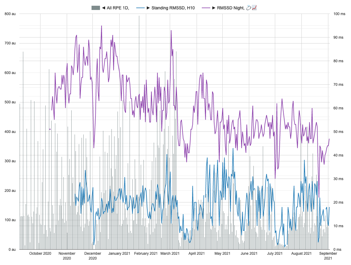
The data summary shown below
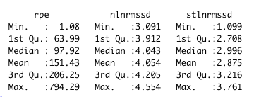
nlnmrssd - nightly ln(RMSSD). stlnmrssd - morning standing ln(RMSSD).rpe - daily sRPE in arbitrary units.
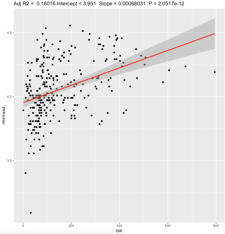
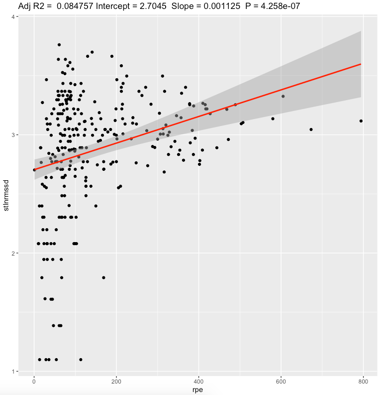
Linear regression, daily sRPE
| effect | p-adjusted | effect size | |
| Nightly ln(RMSSD) | 0.0007 | <0.0001* | moderate |
| Standing ln(RMSSD) | 0.0011 | <0.0001* | weak |
We can see a moderate effect slopes for nightly value and weak effect for standing values. Looking at effect values, standing value seems to have bigger effect value than nightly, but explains less variation of daily sRPE. Both metrics showing that increase in sRPE leads to increase in RMSSD. Confidence intervals are pretty narrow.
Pearson's correlation, daily sRPE
| r | 95% CI | p-adjusted | effect size | |
| Nightly ln(RMSSD) | 0.403 | [0.300,0.497] | <0.0001* | moderate |
| Standing ln(RMSSD) | 0.296 | [0.185,0.400] | <0.0001* | small |
Correlation analysis shows small to moderate correlations for RMSSD. It seems that nightly value have strong relation to daily rpe than standing value.
Discussion
The main result of this experiment is a statistically significant association between HRV and daily physical activity. Nightly values seems to have stronger connection with daily physical activity compared to standing. Positive direction of correlation confirmed for both metrics.
In conclusion, these is a significant connection in positive direction between HRV and physical activity.
Limitations:
- These results are NOT generalizable
- Absence of blinding, randomization, observational nature, n=1
- Often correlation ≠ causation
- Questionnaires widely used in research are prone to participant bias.
- There is a lot of other factors affecting HRV (sleep, diet, caffeine etc) which not taken into account
Data availability & Information
Welcome for questions, suggestions and critics in comments below.
Data is fully available here
library(dplyr)
library(lubridate)
library(effectsize)
library(jsonlite)


ggplotRegression <- function (fit) {

  require(ggplot2)

  ggplot(fit$model, aes_string(x = names(fit$model)[2], y = names(fit$model)[1])) +
    geom_point() +
    stat_smooth(method = "lm", col = "red") +
    labs(title = paste("Adj R2 = ",signif(summary(fit)$adj.r.squared, 5),
                       "Intercept =",signif(fit$coef[[1]],5 ),
                       " Slope =",signif(fit$coef[[2]], 5),
                       " P =",signif(summary(fit)$coef[2,4], 5)))
}


daily <- read.csv("https://blog.kto.to/uploads/pa-na-rpe-sick-food-step-sauna-meditation-hrv.csv")
daily <- daily[!is.na(daily$`sick`),]
daily <- daily[!is.na(daily$`rpe`),]
daily <- daily[!is.na(daily$`rpe7d`),]
daily <- daily[!is.na(daily$`nlnrmssd`),]
daily <- daily[!is.na(daily$`nlnrmssd7d`),]
daily <- daily[!is.na(daily$`stlnrmssd`),]
daily <- daily[!is.na(daily$`stlnrmssd7d`),]

for(i in 1:(nrow(daily)-1))
{
  daily$stlnrmssd[i] = daily$stlnrmssd[i+1]
}

daily <- head(daily,-1)

summary(daily)

l <- lm(cbind(nlnrmssd, stlnrmssd) ~ rpe, data=daily)
summary(daily)
summary(anova(l))
s <- summary(l); s
interpret_r2(s$`Response nlnrmssd`$adj.r.squared[1])
interpret_r2(s$`Response stlnrmssd`$adj.r.squared[1])

p.adjust(c(
  s$`Response nlnrmssd`$coefficients[,4][2],
  s$`Response stlnrmssd`$coefficients[,4][2]
), method="BH")

confint(l , level = 0.05)

ggplotRegression(lm(nlnrmssd ~ rpe, data=daily))
ggplotRegression(lm(stlnrmssd ~ rpe, data=daily))

c <- cor.test(daily$nlnrmssd, daily$rpe); c
interpret_r(c$estimate[[1]][1], "cohen1988")

c <- cor.test(daily$stlnrmssd, daily$rpe); c
interpret_r(c$estimate[[1]][1], "cohen1988")

Response nlnrmssd :

Call:
lm(formula = nlnrmssd ~ rpe, data = daily)

Residuals:
     Min       1Q   Median       3Q      Max
-0.88178 -0.13245 -0.00708  0.12555  0.51767

Coefficients:
             Estimate Std. Error t value Pr(>|t|)
(Intercept) 3.9509776  0.0185872 212.564  < 2e-16 ***
rpe         0.0006803  0.0000924   7.362 2.05e-12 ***
---
Signif. codes:  0 ‘***’ 0.001 ‘**’ 0.01 ‘*’ 0.05 ‘.’ 0.1 ‘ ’ 1

Residual standard error: 0.2047 on 278 degrees of freedom
Multiple R-squared:  0.1632,    Adjusted R-squared:  0.1602
F-statistic: 54.21 on 1 and 278 DF,  p-value: 2.052e-12


Response stlnrmssd :

Call:
lm(formula = stlnrmssd ~ rpe, data = daily)

Residuals:
     Min       1Q   Median       3Q      Max
-1.73344 -0.21062  0.06007  0.31475  0.98806

Coefficients:
             Estimate Std. Error t value Pr(>|t|)
(Intercept) 2.7045107  0.0436854   61.91  < 2e-16 ***
rpe         0.0011250  0.0002172    5.18 4.26e-07 ***
---
Signif. codes:  0 ‘***’ 0.001 ‘**’ 0.01 ‘*’ 0.05 ‘.’ 0.1 ‘ ’ 1

Residual standard error: 0.4812 on 278 degrees of freedom
Multiple R-squared:  0.08804,    Adjusted R-squared:  0.08476
F-statistic: 26.84 on 1 and 278 DF,  p-value: 4.258e-07


> interpret_r2(s$`Response nlnrmssd`$adj.r.squared[1])
[1] "moderate"
(Rules: cohen1988)
> interpret_r2(s$`Response stlnrmssd`$adj.r.squared[1])
[1] "weak"
(Rules: cohen1988)
>
> p.adjust(c(
+   s$`Response nlnrmssd`$coefficients[,4][2],
+   s$`Response stlnrmssd`$coefficients[,4][2]
+ ), method="BH")
         rpe          rpe
4.103419e-12 4.258027e-07
>
> confint(l , level = 0.05)
                            47.5 %       52.5 %
nlnrmssd:(Intercept)  3.9498109795 3.9521441729
nlnrmssd:rpe          0.0006745098 0.0006861088
stlnrmssd:(Intercept) 2.7017688862 2.7072525790
stlnrmssd:rpe         0.0011114168 0.0011386777
>
> c <- cor.test(daily$nlnrmssd, daily$rpe); c

    Pearson's product-moment correlation

data:  daily$nlnrmssd and daily$rpe
t = 7.3625, df = 278, p-value = 2.052e-12
alternative hypothesis: true correlation is not equal to 0
95 percent confidence interval:
 0.3009738 0.4976033
sample estimates:
      cor
0.4039438

> interpret_r(c$estimate[[1]][1], "cohen1988")
[1] "moderate"
(Rules: cohen1988)
>
> c <- cor.test(daily$stlnrmssd, daily$rpe); c

    Pearson's product-moment correlation

data:  daily$stlnrmssd and daily$rpe
t = 5.1804, df = 278, p-value = 4.258e-07
alternative hypothesis: true correlation is not equal to 0
95 percent confidence interval:
 0.1859569 0.4000191
sample estimates:
      cor
0.2967106

> interpret_r(c$estimate[[1]][1], "cohen1988")
[1] "small"
(Rules: cohen1988)
Statistical analysis
RStudio version 1.3.959 and R version 4.0.2 was user for a simple linear regression model and to calculate slopes and p-values.
P-adjusted is p-value adjusted for multiple comparisons by method of Benjamini, Hochberg, and Yekutieli.
Effect sizes based on adjusted R2, Cohen's 1988 rules. Same for Pearson's correlation.