Time Restricted Eating

Time restricted eating (TRE) seems to have good impact on our healt.There is good explanations of scientific background in a Circadian Code book by Satchin Panda. Various studies with TRE as intervention shows promising results in keeping metabolic health in a good shape.

Since i have detailed food log for a long time, i can check what is my usual eating window.

Heatmap of calorie intake by time:

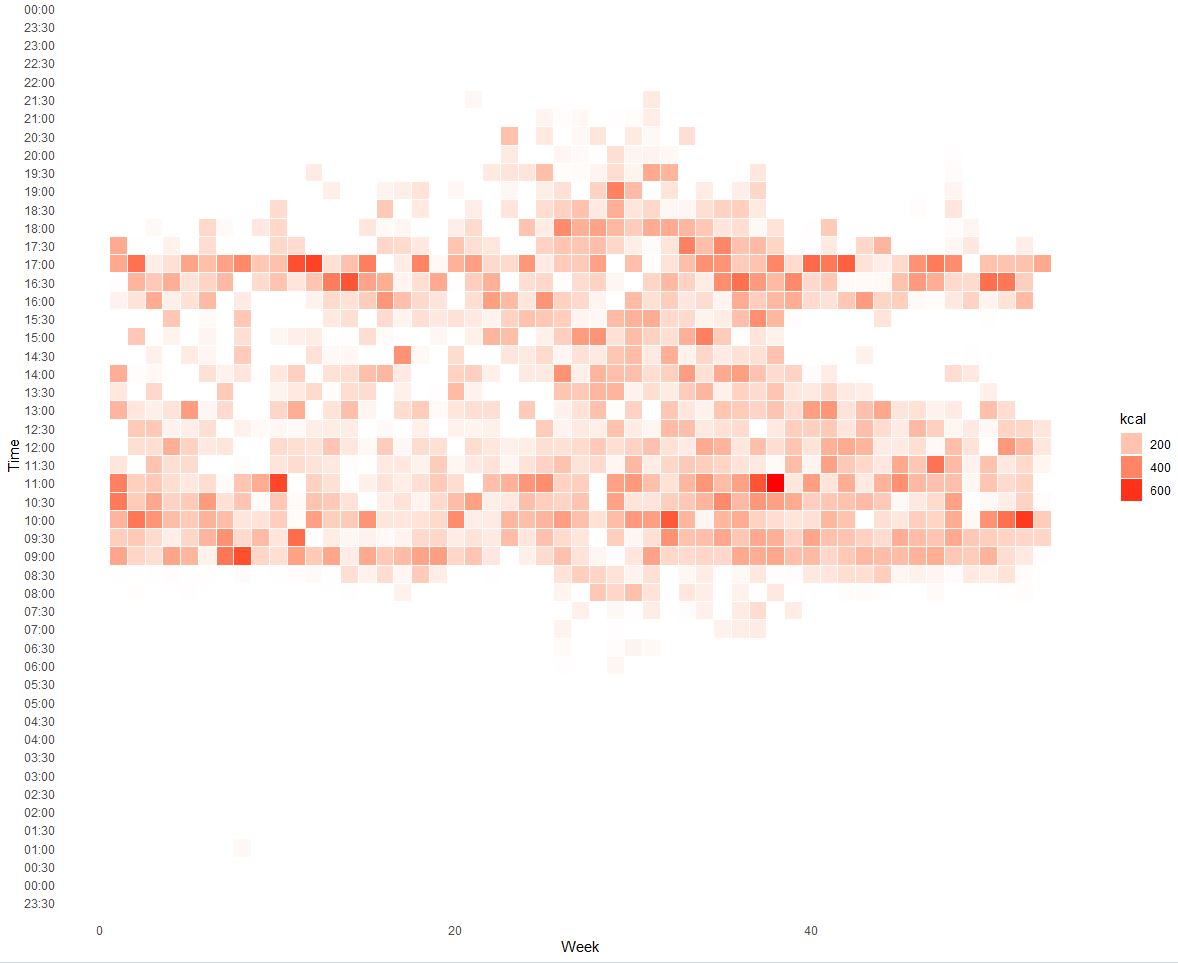
X - week number, Y - time of day, Color - food intake in kcal (sum).

As we can see my usual breakfast time is around 9:00 and dinner before 17:30 which is 8.5 hours average time window and confirms my constant meal regime.

Dailly Glucose

Lets check what is my blood glucose daily pattern looks like:

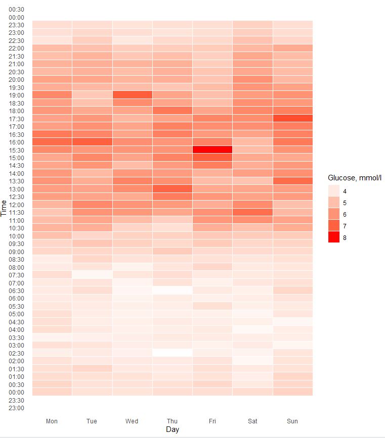
40 days of data grouped by day of week

Optimal dinner time

Even finishing dinner before 17:30 results in postprandial glucose elevation until 21:30-22:00. My usual bedtime start is 22:00-22:30. It seems i should keep my dinner before 17:30 and avoid late meals to make sure my body have enough time to deal with it before i go sleep.

Data availability & Information

Data is available for calorie intake here and for CGM glucose (FreeStyle Libre) here

#Calorie intake

library(lubridate)
library(dplyr)
library(plyr)
library(ggplot2)

df <- read.csv("https://blog.kto.to/uploads/food-kcal.csv")
df <- df[!is.na(df$`kcal`),];

df$ymd <-ymd_hms(df$datetime)
df$date <-as.Date(df$ymd)
df$month <- month(df$datetime, label = TRUE)
df$year <- year(df$datetime)
df$day <- day(df$datetime)
df$week <- week(df$datetime)
df$wday <- wday(df$datetime, label = TRUE)
df$hour <- hour(df$datetime)
df$minute <- 60*60*df$hour + round(minute(df$datetime)/30)*30*60
df$time <- format(as.POSIXct('1900-1-1') + df$minute, '%H:%M:%S')

hdf <- ddply(df, c( "time", "week"), summarise, kcal = sum(kcal)/7)
hdf$x <- hdf$week
#hdf$x <- factor(hdf$month, levels=rev(levels(hdf$month)))
hdf$y <- as.POSIXct(strptime(hdf$time, format = "%H:%M:%S"))
hdf$f <- hdf$kcal

library(scales)

ggplot(hdf, aes(x, y)) + geom_tile(aes(fill = f), colour = "white", na.rm = TRUE) +
  scale_fill_gradient(low = "white", high = "red") +  
  guides(fill=guide_legend(title="kcal")) +
  scale_y_datetime(date_breaks = "30 min", date_labels = "%H:%M") +
  theme_bw() + theme_minimal() +
  labs(title = "Histogram of Food", x = "Week", y = "Time") +
  theme(panel.grid.major = element_blank(), panel.grid.minor = element_blank())\

#Glucose

library(lubridate)
library(dplyr)
library(plyr)
library(ggplot2)

#sleep status for 30 sec periods
df <- read.csv("https://blog.kto.to/uploads/cgm.csv")
df <- df[!is.na(df$`glucose`),];

df$ymd <-ymd_hms(df$datetime)
df$date <-as.Date(df$ymd)
df$month <- month(df$datetime, label = TRUE)
df$year <- year(df$datetime)
df$day <- day(df$datetime)
df$week <- week(df$datetime)
df$wday <- wday(df$datetime, label = TRUE)
df$hour <- hour(df$datetime)
df$minute <- 60*60*df$hour + round(minute(df$datetime)/30)*30*60
df$time <- format(as.POSIXct('1900-1-1') + df$minute, '%H:%M:%S')

hdf <- ddply(df, c( "time", "wday"), summarise, glucose = mean(glucose))
dayLabs<-c("Mon","Tue","Wed","Thu","Fri","Sat","Sun")
hdf$x <- factor(hdf$wday, levels=dayLabs)
hdf$y <- as.POSIXct(strptime(hdf$time, format = "%H:%M:%S"))
hdf$f <- hdf$glucose

library(scales)

ggplot(hdf, aes(x, y)) + geom_tile(aes(fill = f), colour = "white", na.rm = TRUE) +
  scale_fill_gradient(low = "white", high = "red") +  
  guides(fill=guide_legend(title="Glucose, mmol/l")) +
  scale_y_datetime(date_breaks = "30 min", date_labels = "%H:%M") +
  theme_bw() + theme_minimal() +
  labs(title = "Histogram of Sleep", x = "Day", y = "Time") +
  theme(panel.grid.major = element_blank(), panel.grid.minor = element_blank())

Statistical analysis

RStudio version 1.3.959 and R version 4.0.2.