Abstract

What did i do?

I've measured my wrist skin temperature circadian rhythm, to check if it can be distinguished by wrist measures, since iButton test are less comfortable.

How did i do it?

I've used Fitbit Charge 4 placed on wrist to measure skin temperature.

What did i learn?

My body temperature circadian rhythm is present even in Fitbit Charge 4 measurements with 1.67℃ difference and large effect size

Introduction

Circadian rhythm disorders may decrease our healthspan and increase occurrence chronic diseases during aging.

The purpose of this experiment (n=1) is to find diurnal changes in body temperature.

Materials & Methods

Participants

Adult male (n=1) anthropometrics was described in previous article

Experimental design

From 2021-06-01 to 2021-06-28 (28 days) skin temperature was measured by Fitbit Charge 4 placed on wrist 1cm away from bone and wearing it tight enough to have good contact with skin. Fitbit temperature data returned as deviations, not an absolute values.

Results

Visual inspection of data reveals some circadian pattern:

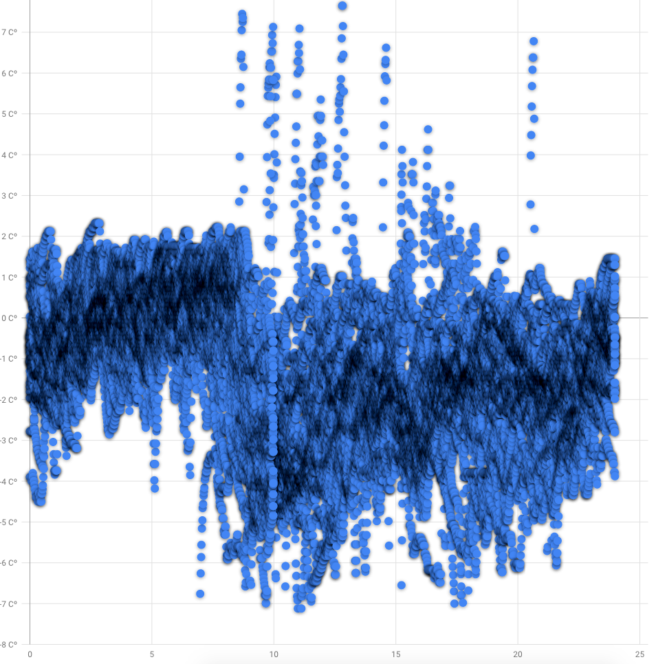
Blue dots is a wrist temperature in celsius. X axis is a hour of day. Google Developer charts for some reasons doesnt show decimal point for temperature and adding empty 25 hour. Measurements density highlighted by shadowing.

Usually, skin temperature have negative correlation to body temperature, resulting in higher temperature at night compared to day and we can clearly see it in visual inspection. But trends arent same as for iButtons body temperature which looks more sinusoidal.

Day vs Night temperature

	Mean	95% CI
Day (9:00 - 19:00)	-2.143℃	[-2.168, -2.119]
Night (21:00 - 7:00)	-0.475℃	[-0.4946, -0.4563]

Confidence intervals a pretty narrow and far away enough to prove statistically significant difference between day and night.

Group differences

	Effect size	95% CI
Hedges g	Large	[1.1233,1.1233]
Mean difference	1.6687℃	[1.6687, 1.6687]

We can see a extremely narrow CI's showing a difference of 1.67℃ between day and night with "Large" effect size.

Discussion

The main result of that experiment is 1.67℃ difference between day and night which acts as a proxy of my circadian rhythm strength. I'll continue checking it in future, to see the trends.

Measuring skin temperature with Fitbit Charge 4 is more convenient compared to iButtons and can be used in long term.

Data availability & Information

Welcome for questions, suggestions and critics in comments below.

Data is fully available here. Original unmodified (exported) raw data is here.

library(goftest)
library(dplyr)
library(effectsize)
library(lubridate)
library(ggplot2)
library(boot)
library(bootES)


ggplotRegression <- function (fit) {
 
  require(ggplot2)
 
  ggplot(fit$model, aes_string(x = names(fit$model)[2], y = names(fit$model)[1])) +
    geom_point() +
    stat_smooth(method = "lm", col = "red") +
    labs(title = paste("Adj R2 = ",signif(summary(fit)$adj.r.squared, 5),
                       "Intercept =",signif(fit$coef[[1]],5 ),
                       " Slope =",signif(fit$coef[[2]], 5),
                       " P =",signif(summary(fit)$coef[2,4], 5)))
}


temp <- read.csv("https://blog.kto.to/uploads/circadian-fitbit.csv")
temp <- temp[!is.na(temp$wristtempdev),]

#filter 21:00 - 7:00 as group 1, 9:00 - 19:00 as group 2, other as group 0
temp <- temp %>% select(datetime,wristtempdev)  %>%
  mutate(group = if_else(((hour(datetime) >= 21) | (hour(datetime) <=  7)), 1,
                         if_else(((hour(datetime) <= 19) & (hour(datetime) >=  9)),2, 0)));

#remove group 0
temp <- temp[temp$group != 0,]

#check for normality distribution
st <-ad.test(temp$wristtempdev) #shapiro.test for n < 5000,  ad.test othervise
if_else(st$p.value < 0.05, 'non-uniform distribution', 'uniform distribution')

bootMean <- function(data, i) { d <- data[i]; return(mean(d)); }
bootMeanDiff <- function(data, i)
{
  d <- data;
  data_group1 <- !is.na(d$group)&d$group == 1
  data_group2 <- !is.na(d$group)&d$group == 2
  g1 <- d$wristtempdev[data_group1]
  g2 <- d$wristtempdev[data_group2]
  return(mean(g1) - mean(g2));
}
bootHedgesG <- function(data, i) #calc hedges G to measure effect sizes
{
  d <- data;
  data_group1 <- !is.na(d$group)&d$group == 1
  data_group2 <- !is.na(d$group)&d$group == 2
  g1 <- d$wristtempdev[data_group1]
  g2 <- d$wristtempdev[data_group2]
  h <- hedges_g(g1, g2)
  return(h$Hedges_g[1]);
}

#bootstrap hedges G effect size between group 1 and 2
results <- boot(data=temp, statistic=bootHedgesG, R=10000)
boot_result <- boot.ci(results, type = c("perc")); boot_result;
interpret_g(1.1233, "cohen1988");

#bootstrap mean difference between group 1 and 2
results <- boot(data=temp, statistic=bootMeanDiff, R=10000)
boot_result <- boot.ci(results, type = c("perc")); boot_result;

#take out group 1 and 2 from dataset
data_group <- !is.na(temp$group)&temp$group == 1
day <- temp$wristtempdev[data_group]

data_group <- !is.na(temp$group)&temp$group == 2
night <- temp$wristtempdev[data_group]

#calc averages & CI
results <- boot(data=day, statistic=bootMean, R=10000)
day_result <- boot.ci(results, type = c("perc")); day_result;

results <- boot(data=night, statistic=bootMean, R=10000)
night_result <- boot.ci(results, type = c("perc")); night_result;

[1] "All values of t are equal to  1.12336690875518 \n Cannot calculate confidence intervals"
NULL

[1] "large"
(Rules: cohen1988)

[1] "All values of t are equal to  1.66875117235629 \n Cannot calculate confidence intervals"
NULL

BOOTSTRAP CONFIDENCE INTERVAL CALCULATIONS
Based on 10000 bootstrap replicates

CALL :
boot.ci(boot.out = results, type = c("perc"))

Intervals :
Level     Percentile     
95%   (-0.4946, -0.4563 )   
Calculations and Intervals on Original Scale

Statistical analysis

RStudio version 1.3.959 and R version 4.0.2. Confidence Intervals was build using bootstrap. Effect sizes based on Hedge's g, Cohen's 1988 rules