Abstract

What did i do?

I've measured my HRV to find out if it correlates with weekly physical activity.

How did i do it?

I've assessed physical activity by using session RPE approach, nightly HRV by using Oura ring and morning standing HRV by using Polar H10.

What did i learn?

There is large positive correlation between weekly HRV and physical activity. Standing values seems to be more sensitive to increased physical activity. 7-day rolling averages provides better insights compared to daily values and strengthens previous findings.

Increase in physical activity leads to increase in HRV as main results of weekly and daily analysis.

Introduction

There is a some evidence that HRV have strong connection with physical activity.

The purpose of this observational data analysis (n=1) is to find if increase in physical activity cause increase in HRV.

Materials & Methods

Participants

Adult male (n=1) anthropometrics was described in previous article

Experimental design

From 2020-09-19 to 2021-09-01 (284 days) daily physical activity was calculated by using sRPE approach, described here. 7-day rolling sum were calculated.

Nightly HRV (RMSSD) was measured by Oura ring on a daily basis. 7-day rolling averages were calculated and log-transformed.

Morning HRV (RMSSD) was measured by Polar H10 in Kubios HRV app, after emptying urinary bladder, within 5 minutes after waking up. Stabilization period was 1 minute and measurement duration was 1 minute. 7-day rolling averages were calculated and log-transformed.

Results

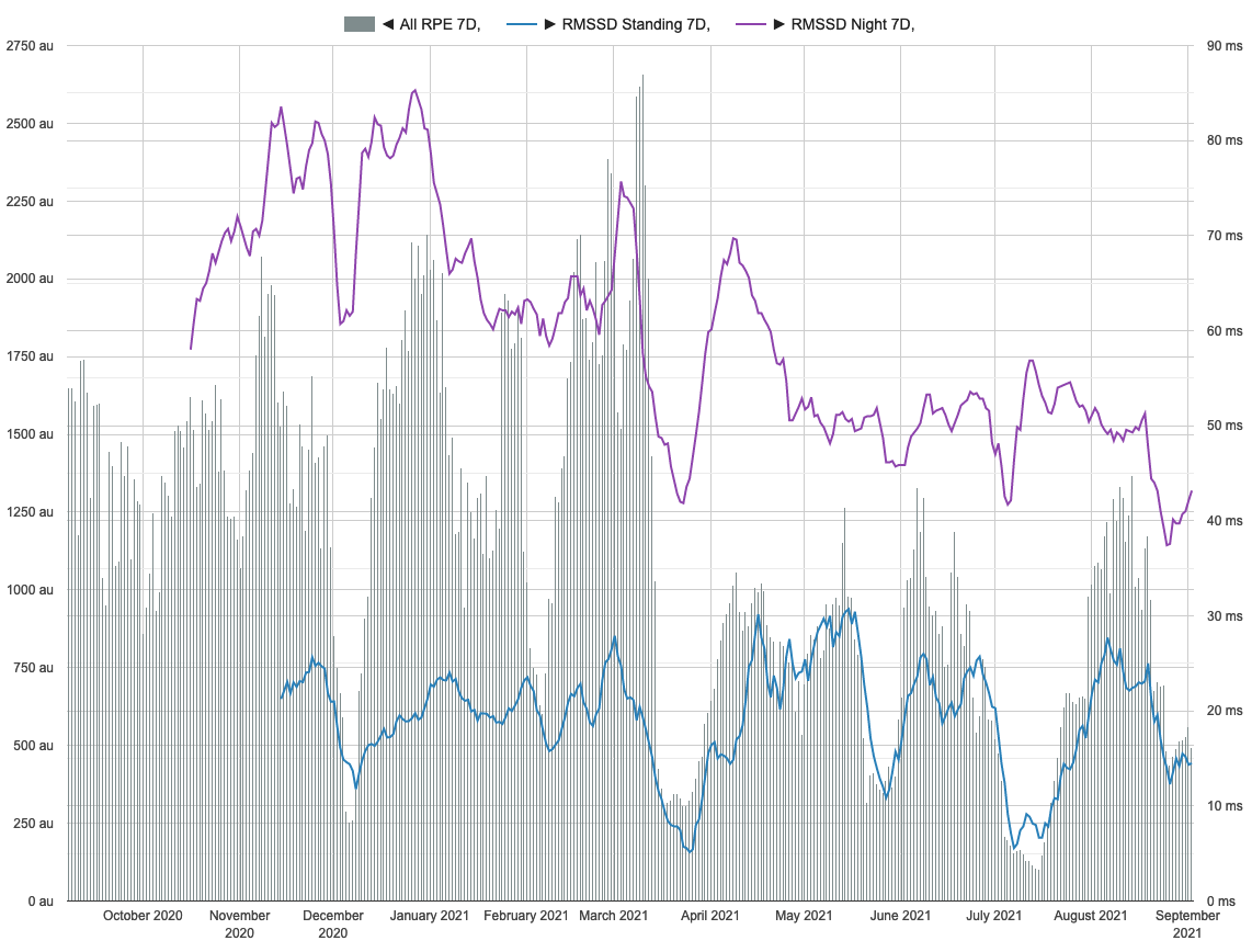
Visual inspection of weekly data is better at revealing connections for metrics  then daily window:

The data summary shown below

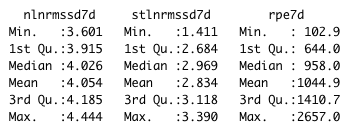
nlnmrssd7d - 7-day rolling average nightly ln(RMSSD). stlnmrssd7d- 7-day rolling average morning standing ln(RMSSD). rpe7d - 7-day rolling sum sRPE in arbitrary units.

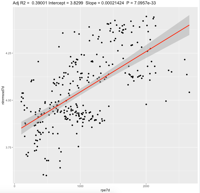
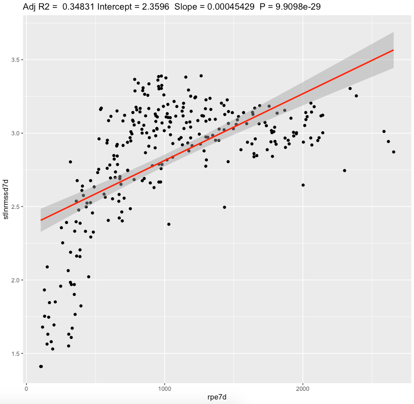
Linear regression, 7-day sRPE

	effect	p-adjusted	effect size
7-day Nightly ln(RMSSD)	0.00021	<0.0001*	substantial
7-day Standing ln(RMSSD)	0.00045	<0.0001*	substantial

We can see a substantial effect slopes for nightly and standing values. Looking at effect values, standing value seems to be more sensitive fo increases in training load. Both metrics showing that increase in sRPE leads to increase in RMSSD. Confidence intervals are pretty narrow. Additional 1-hour training per week with RPE = 6 adds 360au sRPE and increase standing ln(RMSSD) for 500*0.00045 = 0.16 which is equal to ~3ms (+16%)

Pearson's correlation, 7-day sRPE

	r	95% CI	p-adjusted	effect size
7-day Nightly ln(RMSSD)	0.626	[0.550,0.691]	<0.0001*	large
7-day Standing ln(RMSSD)	0.592	[0.511,0.662]	<0.0001*	large

Correlation analysis shows large correlations for both values. Confidence intervals are narrow enough.

Discussion

The main result of this experiment is a statistically significant association between 7-day rolling average HRV and physical activity. Both values show large correlations with standing RMSSD having better sensivity to changes in physical activity.

In conclusion, there is a powerful connection between weekly HRV and physical activity compared to daily values. Increases in weekly training load result in increased HRV.

Limitations:

• These results are NOT generalizable
• Absence of blinding, randomization, observational nature, n=1
• Often correlation ≠ causation
• Questionnaires widely used in research are prone to participant bias.
• There is a lot of other factors affecting HRV (sleep, diet, caffeine etc) which not taken into account

Data availability & Information

Welcome for questions, suggestions and critics in comments below.

Data is fully available here

library(dplyr)
library(lubridate)
library(effectsize)
library(jsonlite)


ggplotRegression <- function (fit) {
 
  require(ggplot2)
 
  ggplot(fit$model, aes_string(x = names(fit$model)[2], y = names(fit$model)[1])) +
    geom_point() +
    stat_smooth(method = "lm", col = "red") +
    labs(title = paste("Adj R2 = ",signif(summary(fit)$adj.r.squared, 5),
                       "Intercept =",signif(fit$coef[[1]],5 ),
                       " Slope =",signif(fit$coef[[2]], 5),
                       " P =",signif(summary(fit)$coef[2,4], 5)))
}



daily <- read.csv("https://blog.kto.to/uploads/pa-na-rpe-sick-food-step-sauna-meditation-hrv.csv")
daily <- daily[!is.na(daily$`rpe7d`),]
daily <- daily[!is.na(daily$`nlnrmssd7d`),]
daily <- daily[!is.na(daily$`stlnrmssd7d`),]

daily$pa = NULL
daily$na = NULL
daily$food = NULL
daily$steps = NULL
daily$sauna = NULL
daily$meditation = NULL
daily$sick = NULL
daily$rpe = NULL
daily$stlnrmssd = NULL
daily$nlnrmssd = NULL
#daily$rpe7d = NULL

for(i in 1:(nrow(daily)-1))
{
  daily$stlnrmssd7d[i] = daily$stlnrmssd7d[i+1]
}

daily <- head(daily,-1)

summary(daily)

l <- lm(cbind(nlnrmssd7d, stlnrmssd7d) ~ rpe7d, data=daily)
summary(anova(l))
s <- summary(l); s
interpret_r2(s$`Response nlnrmssd7d`$adj.r.squared[1])
interpret_r2(s$`Response stlnrmssd7d`$adj.r.squared[1])

p.adjust(c(
  s$`Response nlnrmssd7d`$coefficients[,4][2],
  s$`Response stlnrmssd7d`$coefficients[,4][2]
), method="BH")

confint(l , level = 0.05)

ggplotRegression(lm(nlnrmssd7d ~ rpe7d, data=daily))
ggplotRegression(lm(stlnrmssd7d ~ rpe7d, data=daily))

c <- cor.test(daily$nlnrmssd7d, daily$rpe7d); c
interpret_r(c$estimate[[1]][1], "cohen1988")

c <- cor.test(daily$stlnrmssd7d, daily$rpe7d); c
interpret_r(c$estimate[[1]][1], "cohen1988")

Response nlnrmssd7d :

Call:
lm(formula = nlnrmssd7d ~ rpe7d, data = daily)

Residuals:
    Min      1Q  Median      3Q     Max
-0.3570 -0.1156 -0.0031  0.1248  0.3697

Coefficients:
             Estimate Std. Error t value Pr(>|t|)    
(Intercept) 3.830e+00  1.867e-02  205.12   <2e-16 ***
rpe7d       2.142e-04  1.575e-05   13.61   <2e-16 ***
---
Signif. codes:  0 ‘***’ 0.001 ‘**’ 0.01 ‘*’ 0.05 ‘.’ 0.1 ‘ ’ 1

Residual standard error: 0.1501 on 287 degrees of freedom
Multiple R-squared:  0.3921,    Adjusted R-squared:   0.39
F-statistic: 185.1 on 1 and 287 DF,  p-value: < 2.2e-16


Response stlnrmssd7d :

Call:
lm(formula = stlnrmssd7d ~ rpe7d, data = daily)

Residuals:
    Min      1Q  Median      3Q     Max
-0.9973 -0.2096  0.0289  0.2563  0.6506

Coefficients:
             Estimate Std. Error t value Pr(>|t|)    
(Intercept) 2.3596339  0.0432812   54.52   <2e-16 ***
rpe7d       0.0004543  0.0000365   12.45   <2e-16 ***
---
Signif. codes:  0 ‘***’ 0.001 ‘**’ 0.01 ‘*’ 0.05 ‘.’ 0.1 ‘ ’ 1

Residual standard error: 0.3479 on 287 degrees of freedom
Multiple R-squared:  0.3506,    Adjusted R-squared:  0.3483
F-statistic: 154.9 on 1 and 287 DF,  p-value: < 2.2e-16


> interpret_r2(s$`Response nlnrmssd7d`$adj.r.squared[1])
[1] "substantial"
(Rules: cohen1988)
> interpret_r2(s$`Response stlnrmssd7d`$adj.r.squared[1])
[1] "substantial"
(Rules: cohen1988)
>
> p.adjust(c(
+   s$`Response nlnrmssd7d`$coefficients[,4][2],
+   s$`Response stlnrmssd7d`$coefficients[,4][2]
+ ), method="BH")
       rpe7d        rpe7d
1.419136e-32 9.909802e-29
>
> confint(l , level = 0.05)
                              47.5 %       52.5 %
nlnrmssd7d:(Intercept)  3.8287566502 3.8311003449
nlnrmssd7d:rpe7d        0.0002132489 0.0002152253
stlnrmssd7d:(Intercept) 2.3569174716 2.3623502642
stlnrmssd7d:rpe7d       0.0004519974 0.0004565788
>
> c <- cor.test(daily$nlnrmssd7d, daily$rpe7d); c

    Pearson's product-moment correlation

data:  daily$nlnrmssd7d and daily$rpe7d
t = 13.606, df = 287, p-value < 2.2e-16
alternative hypothesis: true correlation is not equal to 0
95 percent confidence interval:
 0.5506006 0.6916087
sample estimates:
      cor
0.6261986

> interpret_r(c$estimate[[1]][1], "cohen1988")
[1] "large"
(Rules: cohen1988)
>
> c <- cor.test(daily$stlnrmssd7d, daily$rpe7d); c

    Pearson's product-moment correlation

data:  daily$stlnrmssd7d and daily$rpe7d
t = 12.447, df = 287, p-value < 2.2e-16
alternative hypothesis: true correlation is not equal to 0
95 percent confidence interval:
 0.5116630 0.6622272
sample estimates:
      cor
0.5920879

> interpret_r(c$estimate[[1]][1], "cohen1988")
[1] "large"
(Rules: cohen1988)