Abstract
What did i do?
I've measured my food intake, physical activity, positive and negative affects, sickness, sleep quality and quantity to find out how different factors affect my sleep.
How did i do it?
I've measured all variables of interest for ~14 months and there is 115 days with all data present. Days without all metrics present were excluded.
What did i learn?
Caffeine, bedtime start, sickness, vitamin D3 and negative emotions significantly and independently influence my sleep. I'll go into direction of lowering caffeine intake, going sleep earlier, take D3 every other morning, and try to reduce stress. New findings going in same direction with previous findings [1] [2].
Introduction
There is a lof of lifestyle factors which may disrupt or improve sleep quantity and quality.
The purpose of this observational data analysis (n=1) is to determine factors influencing my total sleep time.
Materials & Methods
Participants
1 adult male anthropometrics was described in previous article
Experimental design
During 115 nights (from 2020-08-27 to 2021-09-16) sleep quality and quantity was assessed by Dreem 2 EEG Headband which was validated against gold standard PSG. At same time, all food and fluid intake was carefully logged and measures of intereset were extracted from dietary log. Content of nutrients in each product was determined from a popular online food database - https://nutritiondata.self.com/
Measures of interest: daily calories, protein (cal), fat (cal), carb (cal), animal products (meat, fish, eggs in g), d3 (mcg), b12 (μg), potassium (mcg), magnesium (mcg).
Physical activity was calculated by using sRPE approach, described here.
Positive and Negative affect was measured using PANAS scale, described here.
Sauna and occasional meditation sessions were measured in minutes.
Subjective sleep quality, mood, depression, anxiety, stress, fatigue and sleepiness was assessed by a popular in scientific research questionnaires described in previous experiment
Results
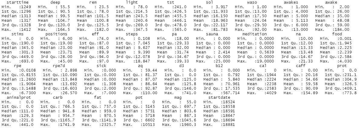
Full dataset summary:
Running simple linear regression with all params versus total sleep time (tst):
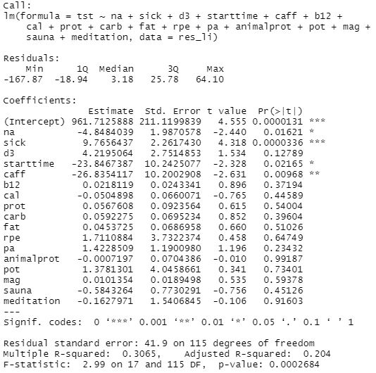
After checking, i've decided to remove non-significant variables. Since d3 isnt far from significance (p-value 0.127), i've decided to keep it. Physical activity, food nutrient structure, b12, potassium & magnesium didnt reveal any connection with a sleep time. That might be because most of my activity falls on the morning / first half of day and i dont eat 3-5 hours prior bed which results in not detectable (small) effects by rough linear analysis or being masked by other influencers not taken into account.
Linear regression after removing non-significant variables:
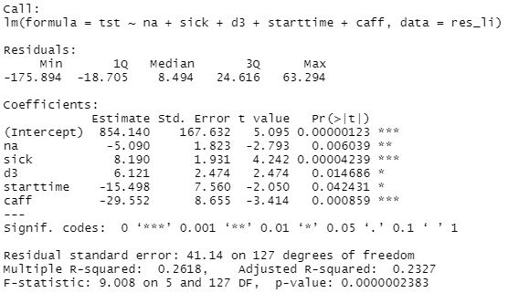
We can see improvements in model: F-statistic increased and R-squared also increased, explaining 23.2% of total sleep time variability.
Linear regression results, Total Sleep Time
| effect, minutes | p-adjusted | ||
| Negative Affect | -5.090 | 0.009* | Worse |
| Sick score | 8.190 | 0.00012* | Better |
| Vitamin D3, per 100 mcg | 6.121 | 0.0176* | Better |
| Bedtime start, h from 00:00 | -15.498 | 0.0424* | Worse |
| Caffeine, per 100 mg | -29.552 | 0.0017* | Worse |
Finally, this model tells:
- 1 additional point of negative affect score decrease my sleep by ~5 minutes
- 1 additional point in sick score increase my sleep by ~8 minutes. My sick score during illness is ~6-8 meaning my sleep during illness is increased by ~1 hour
- supplementing with 125mcg of D3 (5000UI) increases my sleep by ~8 minutes
- bedtime delayed by 1 additional hour decrease my sleep by 15.5 minutes
- 1 starbucks espresso shot (75mg) taken in the morning decrease my sleep by 22 minutes
Discussion
The main result of this experiment is a significant and independent associations between sleep in restorative phases and caffeine, bedtime start, vitamin D3, sickness, negative affect.
Results pointing me to
- lower my caffeine intake to 30mg and strict intake schedule to 8:30 - 10:00.
- go sleep earlier
- supplement with D3 in the morning
- manage negative affect
Checks for linearity, residuals distribution, interaction, collinearity, homoscendasicity, error term correlation seems to indicate acceptable quality of model and explained in Statystical Analysis section.
A limitations:
- These results are NOT generalizable
- Absence of blinding, randomization, observational nature, n=1
- Often correlation ≠ causation
- Questionnaires widely used in research are prone to participant bias.
Statistical Analysis
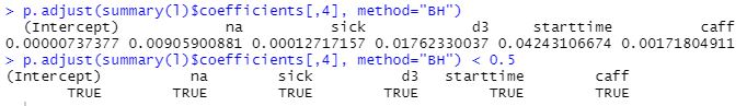
P-values surviving adjusting for multiple comparisons:
The regression lines for each predictor: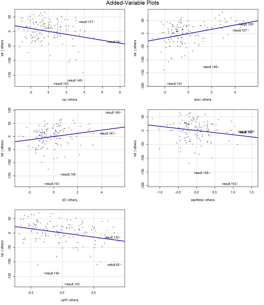
95% Confidence intervals for slopes are narrow enough and Effect size for model is moderate, based on adjusted R-squared. 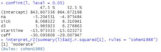
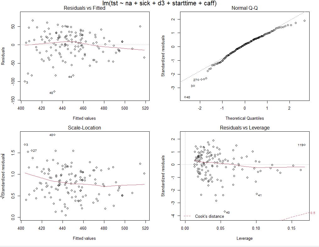
Residuals and their distribution (QQ plot) looks acceptable
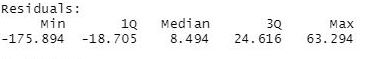
Median of residuals is 8 minutes, not far from 0 and looks acceptable
Model passed test for heteroscendacity, confirms acceptable constant error variance :

Lets check for collinearity in variables of interest:
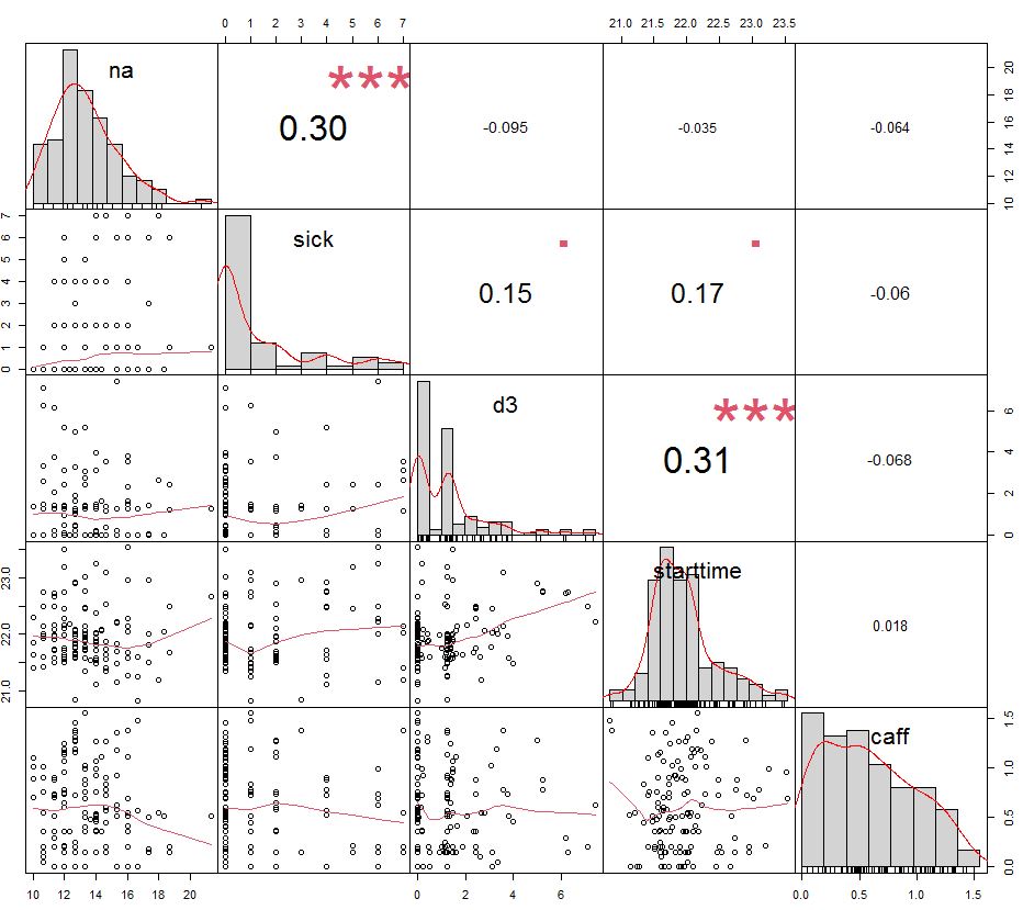
We can see a correlations between sick and negative affect and between d3 and starttime. Lets try to account for their potential interaction and see if model is improved or explained something new: (tst ~ na + sick + sick*na + d3 + starttime + d3*starttime + caff) results in F-statistic 6.847 and shows no improvement, indicating that (tst ~ na + sick + d3 + starttime + caff) with F = 9 is better.
Lets do a final statistical test for collinearity by checking if VIF (variance inflation factor) for each predictor is less than 10
VIF test makes me confident in abscense of collinearity which is good sign for a model.
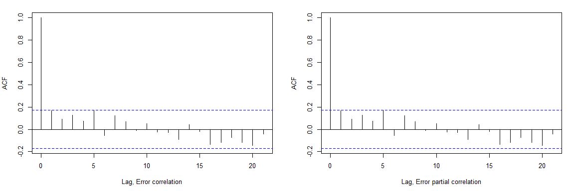
We can see slight autocorrelation for error term, but it looks acceptable
Data availability & Information
Welcome for questions, suggestions and critics in comments below.
Dreem 2 device unmodified data is fully available here and format is explained by manufacturer.
Daily data available here.
R Code:
library(effectsize)
library(splusTimeDate)
library(lubridate)
library(ggplot2)
library(foreach)
library(iterators)
library(skimr)
library(parallel)
library(doParallel)
library(PerformanceAnalytics)
library(car)
library(mctest)
library(ppcor)
library(corpcor)
library(lmtest)

library(mise)
mise()

registerDoParallel(cores=24)
options(scipen = 999)
alpha <- 0.05

daily <- read.csv("https://blog.kto.to/uploads/sleepv2-daily.csv")
#daily <- daily[!is.na(daily$`cal`),]
#daily <- daily[!is.na(daily$`pa`),]
#daily <- daily[!is.na(daily$`rpe`),]
daily <- daily[!is.na(daily$`na`),]
daily <- daily[!is.na(daily$`sick`),]
#daily <- daily[!is.na(daily$`food`),]
#daily <- daily[!is.na(daily$`steps`),]
daily$`sauna`[is.na(daily$`sauna`)] <- 0;
daily$`animalprot`[is.na(daily$`animalprot`)] <- 0;
daily$`mag`[is.na(daily$`mag`)] <- 0;
daily$`pot`[is.na(daily$`pot`)] <- 0;
daily$`d3`[is.na(daily$`d3`)] <- 0;
daily$`caff`[is.na(daily$`caff`)] <- 0;
daily$`b12`[is.na(daily$`b12`)] <- 0;
daily$`meditation`[is.na(daily$`meditation`)] <- 0;
#row.names(daily) <- NULL

dreem <- read.csv("https://blog.kto.to/uploads/sleepv2-dreem.csv", skip = 5, sep = ';', header = TRUE)
dreem <- dreem[!is.na(dreem$Type),]

results <- foreach(i=1:nrow(dreem), .combine='rbind', .multicombine=TRUE, .packages = "lubridate") %dopar% {
  sleepstart <- strsplit(dreem$Start.Time[i], "T")[[1]][2]
  sleepstartdate <- strsplit(dreem$Start.Time[i], "T")[[1]][1]
  resulted = c();
  for(j in 1:nrow(daily))
  {
    #if((as.Date(daily$datetime[j]) +days(1)) == as.Date(sleepstartdate))
    if((as.Date(daily$datetime[j])) == as.Date(sleepstartdate))
    {
      sleepstarttime <- strsplit(sleepstart, "\\+")[[1]][1]
      if((!is.na(daily$steps[j])))
      {
        resulted <- c(resulted, c(
          starttime = period_to_seconds(hms(sleepstarttime))/60,
          deep = period_to_seconds(hms(dreem$Deep.Sleep.Duration[i]))/60,
          rem = period_to_seconds(hms(dreem$REM.Duration[i]))/60,
          light = period_to_seconds(hms(dreem$Light.Sleep.Duration[i]))/60,
          tst = (period_to_seconds(hms(dreem$Deep.Sleep.Duration[i])) + period_to_seconds(hms(dreem$REM.Duration[i])) + period_to_seconds(hms(dreem$Light.Sleep.Duration[i])))/60,
          sol = period_to_seconds(hms(dreem$Sleep.Onset.Duration[i]))/60,
          waso  = period_to_seconds(hms(dreem$Wake.After.Sleep.Onset.Duration[i]))/60,
          awakes  = dreem$Number.of.awakenings[i],
          awake = period_to_seconds(hms(dreem$Wake.After.Sleep.Onset.Duration[i]))/60 + period_to_seconds(hms(dreem$Wake.After.Sleep.Onset.Duration[i]))/60,
          stims = dreem$Number.of.Stimulations[i],
          positions = dreem$Position.Changes[i],
          eff = dreem$Sleep.efficiency[i],
          steps = daily$steps[j]/1000,
          pa = daily$pa[j],
          sauna = daily$sauna[j],
          meditation = daily$meditation[j],
          na = daily$na[j],
          food = daily$food[j]/1000,
          rpe = daily$rpe[j]/100,
          rpe7d = daily$rpe7d[j]/100,
          sick = daily$sick[j],
          zq = 8.5*((((period_to_seconds(hms(dreem$Deep.Sleep.Duration[i])) + period_to_seconds(hms(dreem$REM.Duration[i])) + period_to_seconds(hms(dreem$Light.Sleep.Duration[i])))/3600)*1) + (0.5*(period_to_seconds(hms(dreem$REM.Duration[i]))/3600) + 1.5*(period_to_seconds(hms(dreem$Deep.Sleep.Duration[i]))/3600)) - ((period_to_seconds(hms(dreem$Wake.After.Sleep.Onset.Duration[i]))/3600+period_to_seconds(hms(dreem$Sleep.Onset.Duration[i]))/3600)*0.5 + dreem$Number.of.awakenings[i]/15)),
          d3 = daily$d3[j],
          b12 = daily$b12[j],
          cal = daily$cal[j],
          caff = daily$caff[j],
          prot = daily$prot[j],
          animalprot = daily$animalprot[j],
          carb = daily$carb[j],
          fat = daily$fat[j],
          pot = daily$pot[j],
          mag = daily$mag[j],
          startdate = as.Date(sleepstartdate)
        ))
      }
    }
  }
  return(c(resulted))
}

res_li <- as.data.frame(results)
row.names(res_li) <- NULL
summary(res_li)

res_li$d3 <- res_li$d3/100
res_li$pot <- res_li$pot/1000
res_li$caff <- res_li$caff/100
res_li$starttime <- res_li$starttime/60

#plat responce variable
plot(as_date(res_li$startdate, origin = lubridate::origin), res_li$tst)

#l <- lm(tst ~ na + sick + d3 + starttime + caff + b12 + cal + prot + carb + fat + rpe + pa + animalprot + pot + mag + sauna + meditation, data=res_li); s <- summary(l); s
l <- lm(tst ~ na + sick + d3 + starttime + caff, data=res_li); s <- summary(l); s
summary(anova(l))
mse <- mean(residuals(l)^2); mse
rss <- sum(residuals(l)^2); rss
rse <- sqrt(rss / l$df.residual); rse

#Effect size for R^2
interpret_r2(summary(l)$adj.r.squared[1], rules = "cohen1988")

#1 adjust p-values for multiple comparisons
p.adjust(summary(l)$coefficients[,4], method="BH") < alpha
confint(l, level = alpha)

print("1. Verification of Lineriaty: check each predictor")
#inspect each predictor
avPlots(l)

print("2. Verification of interaction: remove additive/interaction assumption")
#if F/T-statistics are improved, there might be an interaction
#check for interactions p-values. multiplication and both interaction predictors must be included!
la <- lm(tst ~ na + sick + (na * sick) + d3 + starttime + (d3 * starttime) + caff, data=res_li); s <- summary(la); s
la <- lm(tst ~ na + sick + d3 + starttime + (d3 * starttime) + caff, data=res_li); s <- summary(la);  s
la <- lm(tst ~ na + sick + (na * sick) + d3 + starttime + caff, data=res_li); s <- summary(la);  s

print("3. Verification of Residuals: check linearity of residuals and non-constant error variance (heteroscedasticity)")
#Linear fit. Red residual line should be linear horizontal on Residual vs Fitted
#Homoscedasticity : Residual vs Fitted and Scale-Location. Completely random, equal distribution is required to confirm Homoscedasticity
par(mfrow = c(2,2)); plot(l)
car::ncvTest(l)$p < alpha #TRUE indicates Homoscedasticity

print("4. Verification of Error term correlation")
acf(l$residuals, main="Error term correlation")
acf(l$residuals, main="Error term partial correlation")

print("5. Remove Outliers and re-check model")
cooksD <- cooks.distance(l)
influential <- cooksD[(cooksD > (20 * mean(cooksD, na.rm = TRUE)))]
names_of_influential <- names(influential)
res_li_no_outliers <- res_li[-c(as.numeric(names(influential))),]
lno <- lm(tst ~ na + sick + d3 + starttime + caff, data=res_li_no_outliers); s <- summary(lno); s
p.adjust(summary(lno)$coefficients[,4], method="BH") < alpha
par(mfrow = c(2,2)); plot(lno)
car::ncvTest(lno)$p < alpha #TRUE indicates Homoscedasticity
l <- lno

print("6. Verification of Collinearity: predictors shouldn't have collinearity")
print("Collinearity #1: visual examination (paired)")

#look at correlation chart
rl <- list(res_li$na, res_li$sick, res_li$d3, res_li$starttime, res_li$caff)
names(rl) <- c("na","sick","d3","starttime","caff")
chart.Correlation(as.data.frame(rl), histogram = TRUE, method = "pearson")

#look p-val < alpha
print("Collinearity #2 check for p-values for correlations")
pvalcor <- pcor(as.data.frame(rl), method = "pearson"); diag(pvalcor$p.value) <- NA;  diag(pvalcor$estimate) <- NA
round(pvalcor$estimate,2)
pvalcor$p.value < alpha

#look for partical correlation table
print("Collinearity #3: check partial correlation which take into account other predictors")
partialcor <- cor2pcor(cov(as.data.frame(rl))); diag(partialcor) <- NA
round(partialcor,2)

print("Collinearity #4: check variance inflation factor (for MLM). if VIF > 10 then collinearity is detected")
omcdiag(l, Inter = TRUE)
imcdiag(l, method = "VIF")$idiags[,1] > 10
Statistical analysis
RStudio version 1.3.959 and R version 4.0.2 was user for a multiple linear regression model and to calculate slopes and p-values.
P-adjusted is p-value adjusted for multiple comparisons by method of Benjamini, Hochberg, and Yekutieli.
Effect sizes based on adjusted R2, Cohen's 1988 rules
TODO: deeper check for correlation of error terms, outliers, non-constant variance of error terms, high-leverage points and collinearity.